Convergence in τ

Go back to the Contents page.

---

Press Show to reveal the code chunks.

---

Let us set some global options for all code chunks in this document.

# Create a clipboard button
source(here::here("clipboard.R")); clipboard

# Set seed for reproducibility
set.seed(1982) 
# Set global options for all code chunks
knitr::opts_chunk$set(
  # Disable messages printed by R code chunks
  message = FALSE,    
  # Disable warnings printed by R code chunks
  warning = FALSE,    
  # Show R code within code chunks in output
  echo = TRUE,        
  # Include both R code and its results in output
  include = TRUE,     
  # Evaluate R code chunks
  eval = TRUE,       
  # Enable caching of R code chunks for faster rendering
  cache = FALSE,      
  # Align figures in the center of the output
  fig.align = "center",
  # Enable retina display for high-resolution figures
  retina = 2,
  # Show errors in the output instead of stopping rendering
  error = TRUE,
  # Do not collapse code and output into a single block
  collapse = FALSE
)
# Start the figure counter
fig_count <- 0
# Define the captioner function
captioner <- function(caption) {
  fig_count <<- fig_count + 1
  paste0("Figure ", fig_count, ": ", caption)
}

To observe convergence in \(\tau\), we calibrate \(h\) and \(m\) to \(\tau\) as \(h \sim \tau^{1/\alpha}\) and \(m \sim \lceil\log_e^2(h)/(\pi^2(1-\alpha/2))\rceil\), respectively. Under this scaling, the total convergence rate with respect to the time step \(\tau\) is of order \(1\). That is, \(\|u-U_{h,m}^\tau\|_{L_2((0,T);L_2(\Gamma))} \leq C_\tau\tau\). This can be verified by estimating the slope \(S_\tau\) in the regression \(\log_{10} E = S_\tau\log_{10} \tau + \log_{10} C_\tau\), where we expect \(S_\tau\sim1\).

# remotes::install_github("davidbolin/rspde", ref = "devel")
# remotes::install_github("davidbolin/metricgraph", ref = "devel")
library(rSPDE)
library(MetricGraph)
library(grateful)

library(ggplot2)
library(reshape2)
library(plotly)
library(slackr)
source("keys.R")
slackr_setup(token = token) # token comes from keys.R

## [1] "Successfully connected to Slack"

capture.output(
  knitr::purl(here::here("functionality.Rmd"), output = here::here("functionality.R")),
  file = here::here("purl_log.txt")
)
source(here::here("functionality.R"))

# Parameters
T_final <- 2
kappa <- 4
N_finite = 4 # choose even
adjusted_N_finite <- N_finite + N_finite/2 + 1
# Coefficients for u_0 and f
coeff_U_0 <- 50*(1:adjusted_N_finite)^-1
coeff_U_0[-5] <- 0
coeff_FF <- rep(0, adjusted_N_finite)
coeff_FF[7] <- 10

AAA = 1
OMEGA = pi

# Time step and mesh size
POWERS <- seq(6.125, 5.625, by = -0.1)
tau_vector <- 0.1 * 2^-POWERS
alpha_vector <- seq(1, 1.8, by = 0.2)

# Overkill parameters
overkill_time_step <- 0.1 * 2^-14
overkill_h <- (0.1 * 2^-14)^(1/2)
# Finest time and space mesh
overkill_time_seq <- seq(0, T_final, length.out = ((T_final - 0) / overkill_time_step + 1))
overkill_graph <- gets.graph.tadpole(h = overkill_h)
# Compute the weights on the finest mesh
overkill_graph$compute_fem() # This is needed to compute the weights
overkill_C <- overkill_graph$mesh$C
m_values <- c()

# Create a matrix to store the errors
errors_projected <- matrix(NA, nrow = length(tau_vector), ncol = length(alpha_vector))
for (j in 1:length(alpha_vector)) {
  alpha <- alpha_vector[j] # from 0.5 to 2
  beta <- alpha / 2

  # Compute the eigenvalues and eigenfunctions on the finest mesh
  overkill_eigen_params <- gets.eigen.params(N_finite = N_finite, kappa = kappa, alpha = alpha, graph = overkill_graph)
  EIGENVAL_ALPHA <- overkill_eigen_params$EIGENVAL_ALPHA # Eigenvalues (they are independent of the meshes)
  overkill_EIGENFUN <- overkill_eigen_params$EIGENFUN # Eigenfunctions on the finest mesh
  
  # Compute the true solution on the finest mesh
  overkill_U_true <- overkill_EIGENFUN %*% 
    outer(1:length(coeff_U_0), 
          1:length(overkill_time_seq), 
          function(i, j) (coeff_U_0[i] + coeff_FF[i] * G_sin(t = overkill_time_seq[j], A = AAA, lambda_j_alpha_half = EIGENVAL_ALPHA[i], omega = OMEGA)) * exp(-EIGENVAL_ALPHA[i] * overkill_time_seq[j]))
  
  for (i in 1:length(tau_vector)) {
    time_step <- tau_vector[i]
    h <- time_step^(1/alpha)
    m <- min(4, ceiling((log(h))^2 / (pi^2 * (1 - alpha / 2)))) 
    #h <- largest_nested_h(h_star, h) # this makes the spatial mesh nested
    m_values <- c(m_values, m)
    graph <- gets.graph.tadpole(h = h)
    graph$compute_fem()
    G <- graph$mesh$G
    C <- graph$mesh$C
    L <- kappa^2*C + G
    eigen_params <- gets.eigen.params(N_finite = N_finite, kappa = kappa, alpha = alpha, graph = graph)
    EIGENFUN <- eigen_params$EIGENFUN
    U_0 <- EIGENFUN %*% coeff_U_0 # Compute U_0 on the current mesh
    Psi <- graph$fem_basis(overkill_graph$get_mesh_locations())
  
    time_seq <- seq(0, T_final, length.out = ((T_final - 0) / time_step + 1))
    my_op_frac <- my.fractional.operators.frac(L, beta, C, scale.factor = kappa^2, m = m, time_step)
    INT_BASIS_EIGEN <- t(overkill_EIGENFUN) %*% overkill_C %*% Psi
    # Compute matrix F with columns F^k
    FF_approx <- t(INT_BASIS_EIGEN) %*% 
      outer(1:length(coeff_FF), 
            1:length(time_seq), 
        function(i, j) coeff_FF[i] * g_sin(r = time_seq[j], A = AAA, omega = OMEGA))
    
    U_approx <- solve_fractional_evolution(my_op_frac, time_step, time_seq, val_at_0 = U_0, RHST = FF_approx)
    projected_U_approx <- Psi %*% U_approx
    projected_U_piecewise <- construct_piecewise_projection(projected_U_approx, time_seq, overkill_time_seq)
    XX <- overkill_U_true - projected_U_piecewise
    errors_projected[i,j] <- sqrt(as.double(overkill_time_step * sum(XX * (overkill_C %*% XX)))) 
    slackr_msg(text = paste0("m =", m, ", alpha =", alpha, ", h =", h, ", time_step =", time_step), channel = "#research")
  }
}
save(errors_projected, file = here::here("data_files/errors_projected_tau.RData"))

# Load the errors_projected data
load(here::here("data_files/errors_projected_tau.RData"))

observed_rates <- numeric(length(alpha_vector))
for (u in 1:length(alpha_vector)) {
  observed_rates[u] <- coef(lm(log10(errors_projected[, u]) ~ log10(tau_vector)))[2]
}

theoretical_rates <- rep(1, length(alpha_vector))


p_tau <- error.convergence.plotter(x_axis_vector = tau_vector, 
                                   alpha_vector, 
                                   errors_projected, 
                                   theoretical_rates, 
                                   observed_rates,
                                   line_equation_fun = loglog_line_equation,
                                   fig_title = expression("Convergence in " * italic(tau)),
                                   x_axis_label = expression(italic(tau)))
p_tau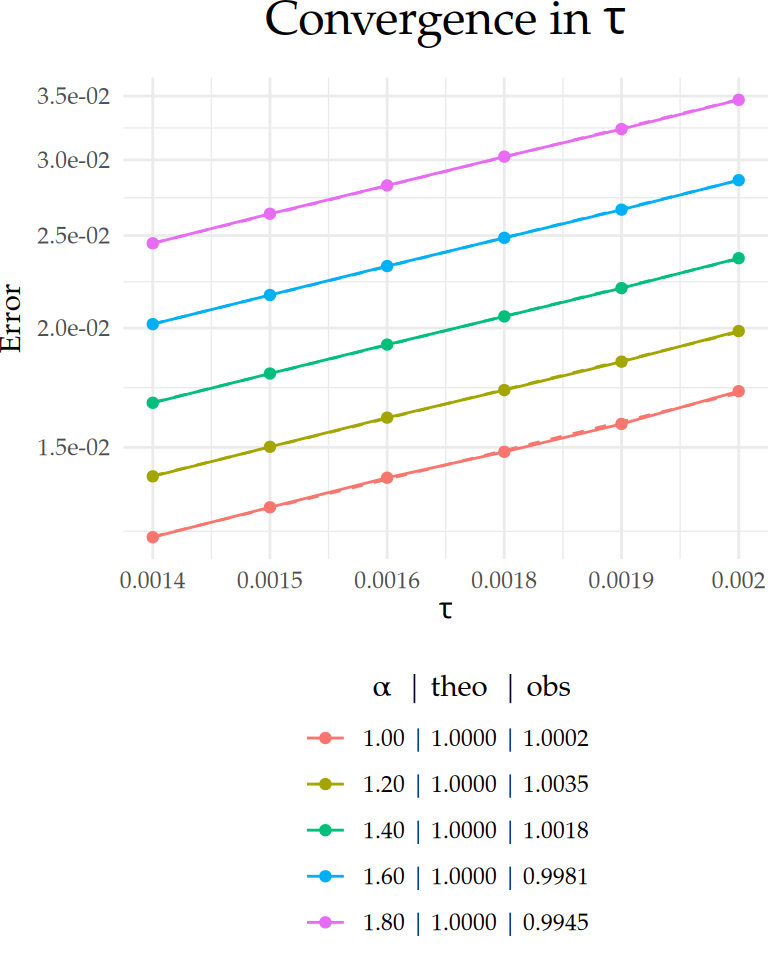

Figure 1: Comparison between theoretical and observed convergence behavior for the \(L_2(\Gamma\times(0,T))\)-error with respect to \(\tau\) on a \(\text{log}_{10}\)–\(\text{log}_{10}\) scale. Dashed lines indicate the theoretical rates, and solid lines represent the observed error curves. The legend below each plot shows the value of \(\alpha\) along with the corresponding theoretical (‘theo’), and observed (‘obs’) rates for each case.

ggsave(here::here("data_files/conv_rates_tau.png"), width = 4, height = 5, plot = p_tau, dpi = 300)
save(p_tau, file = here::here("data_files/p_tau.RData"))

1 References

cite_packages(output = "paragraph", out.dir = ".")

We used R version 4.5.2 (R Core Team 2025) and the following R packages: akima v. 0.6.3.6 (Akima and Gebhardt 2025), expm v. 1.0.0 (Maechler, Dutang, and Goulet 2024), fmesher v. 0.5.0 (Lindgren 2025), gsignal v. 0.3.7 (Van Boxtel, G.J.M., et al. 2021), here v. 1.0.1 (Müller 2020), htmltools v. 0.5.8.1 (Cheng et al. 2024), INLA v. 25.11.22 (Rue, Martino, and Chopin 2009; Lindgren, Rue, and Lindström 2011; Martins et al. 2013; Lindgren and Rue 2015; De Coninck et al. 2016; Rue et al. 2017; Verbosio et al. 2017; Bakka et al. 2018; Kourounis, Fuchs, and Schenk 2018), inlabru v. 2.13.0 (Yuan et al. 2017; Bachl et al. 2019), knitr v. 1.50 (Xie 2014, 2015, 2025a), Matrix v. 1.7.3 (Bates, Maechler, and Jagan 2025), MetricGraph v. 1.5.0.9000 (Bolin, Simas, and Wallin 2023a, 2023b, 2024, 2025; Bolin et al. 2024), neuralnet v. 1.44.2 (Fritsch, Guenther, and Wright 2019), orthopolynom v. 1.0.6.1 (Novomestky 2022), patchwork v. 1.3.1 (Pedersen 2025), pbmcapply v. 1.5.1 (Kuang, Kong, and Napolitano 2022), plotly v. 4.11.0 (Sievert 2020), posterdown v. 1.0 (Thorne 2019), pracma v. 2.4.4 (Borchers 2023), qrcode v. 0.3.0 (Onkelinx and Teh 2024), RColorBrewer v. 1.1.3 (Neuwirth 2022), RefManageR v. 1.4.0 (McLean 2014, 2017), renv v. 1.1.5 (Ushey and Wickham 2025), reshape2 v. 1.4.4 (Wickham 2007), reticulate v. 1.44.1 (Ushey, Allaire, and Tang 2025), rmarkdown v. 2.30 (Xie, Allaire, and Grolemund 2018; Xie, Dervieux, and Riederer 2020; Allaire et al. 2025), rSPDE v. 2.5.1.9000 (Bolin and Kirchner 2020; Bolin and Simas 2023; Bolin, Simas, and Xiong 2024), RSpectra v. 0.16.2 (Qiu and Mei 2024), scales v. 1.4.0 (Wickham, Pedersen, and Seidel 2025), slackr v. 3.4.0 (Kaye et al. 2025), tidyverse v. 2.0.0 (Wickham et al. 2019), viridisLite v. 0.4.2 (Garnier et al. 2023), xaringan v. 0.31 (Xie 2025b), xaringanExtra v. 0.8.0 (Aden-Buie and Warkentin 2024), xaringanthemer v. 0.4.4 (Aden-Buie 2025).

Aden-Buie, Garrick. 2025. xaringanthemer: Custom “xaringan” CSS Themes. https://doi.org/10.32614/CRAN.package.xaringanthemer.

Aden-Buie, Garrick, and Matthew T. Warkentin. 2024. xaringanExtra: Extras and Extensions for “xaringan” Slides. https://doi.org/10.32614/CRAN.package.xaringanExtra.

Akima, Hiroshi, and Albrecht Gebhardt. 2025. akima: Interpolation of Irregularly and Regularly Spaced Data. https://doi.org/10.32614/CRAN.package.akima.

Allaire, JJ, Yihui Xie, Christophe Dervieux, Jonathan McPherson, Javier Luraschi, Kevin Ushey, Aron Atkins, et al. 2025. rmarkdown: Dynamic Documents for r. https://github.com/rstudio/rmarkdown.

Bachl, Fabian E., Finn Lindgren, David L. Borchers, and Janine B. Illian. 2019. “inlabru: An R Package for Bayesian Spatial Modelling from Ecological Survey Data.” Methods in Ecology and Evolution 10: 760–66. https://doi.org/10.1111/2041-210X.13168.

Bakka, Haakon, Håvard Rue, Geir-Arne Fuglstad, Andrea I. Riebler, David Bolin, Janine Illian, Elias Krainski, Daniel P. Simpson, and Finn K. Lindgren. 2018. “Spatial Modelling with INLA: A Review.” WIRES (Invited Extended Review) xx (Feb): xx–. http://arxiv.org/abs/1802.06350.

Bates, Douglas, Martin Maechler, and Mikael Jagan. 2025. Matrix: Sparse and Dense Matrix Classes and Methods. https://doi.org/10.32614/CRAN.package.Matrix.

Bolin, David, and Kristin Kirchner. 2020. “The Rational SPDE Approach for Gaussian Random Fields with General Smoothness.” Journal of Computational and Graphical Statistics 29 (2): 274–85. https://doi.org/10.1080/10618600.2019.1665537.

Bolin, David, Mihály Kovács, Vivek Kumar, and Alexandre B. Simas. 2024. “Regularity and Numerical Approximation of Fractional Elliptic Differential Equations on Compact Metric Graphs.” Mathematics of Computation 93 (349): 2439–72. https://doi.org/10.1090/mcom/3929.

Bolin, David, and Alexandre B. Simas. 2023. rSPDE: Rational Approximations of Fractional Stochastic Partial Differential Equations. https://CRAN.R-project.org/package=rSPDE.

Bolin, David, Alexandre B. Simas, and Jonas Wallin. 2023a. MetricGraph: Random Fields on Metric Graphs. https://CRAN.R-project.org/package=MetricGraph.

———. 2023b. “Statistical Inference for Gaussian Whittle-Matérn Fields on Metric Graphs.” arXiv Preprint arXiv:2304.10372. https://doi.org/10.48550/arXiv.2304.10372.

———. 2024. “Gaussian Whittle-Matérn Fields on Metric Graphs.” Bernoulli 30 (2): 1611–39. https://doi.org/10.3150/23-BEJ1647.

———. 2025. “Markov Properties of Gaussian Random Fields on Compact Metric Graphs.” Bernoulli. https://doi.org/10.48550/arXiv.2304.03190.

Bolin, David, Alexandre B. Simas, and Zhen Xiong. 2024. “Covariance-Based Rational Approximations of Fractional SPDEs for Computationally Efficient Bayesian Inference.” Journal of Computational and Graphical Statistics 33 (1): 64–74. https://doi.org/10.1080/10618600.2023.2231051.

Borchers, Hans W. 2023. pracma: Practical Numerical Math Functions. https://doi.org/10.32614/CRAN.package.pracma.

Cheng, Joe, Carson Sievert, Barret Schloerke, Winston Chang, Yihui Xie, and Jeff Allen. 2024. htmltools: Tools for HTML. https://github.com/rstudio/htmltools.

De Coninck, Arne, Bernard De Baets, Drosos Kourounis, Fabio Verbosio, Olaf Schenk, Steven Maenhout, and Jan Fostier. 2016. “Needles: Toward Large-Scale Genomic Prediction with Marker-by-Environment Interaction.” Genetics 203 (1): 543–55. https://doi.org/10.1534/genetics.115.179887.

Fritsch, Stefan, Frauke Guenther, and Marvin N. Wright. 2019. neuralnet: Training of Neural Networks. https://doi.org/10.32614/CRAN.package.neuralnet.

Garnier, Simon, Ross, Noam, Rudis, Robert, Camargo, et al. 2023. viridis(Lite) - Colorblind-Friendly Color Maps for r. https://doi.org/10.5281/zenodo.4678327.

Kaye, Matt, Bob Rudis, Andrie de Vries, and Jonathan Sidi. 2025. slackr: Send Messages, Images, r Objects and Files to “Slack” Channels/Users. https://github.com/mrkaye97/slackr.

Kourounis, D., A. Fuchs, and O. Schenk. 2018. “Towards the Next Generation of Multiperiod Optimal Power Flow Solvers.” IEEE Transactions on Power Systems PP (99): 1–10. https://doi.org/10.1109/TPWRS.2017.2789187.

Kuang, Kevin, Quyu Kong, and Francesco Napolitano. 2022. pbmcapply: Tracking the Progress of Mc*pply with Progress Bar. https://doi.org/10.32614/CRAN.package.pbmcapply.

Lindgren, Finn. 2025. fmesher: Triangle Meshes and Related Geometry Tools. https://github.com/inlabru-org/fmesher.

Lindgren, Finn, and Håvard Rue. 2015. “Bayesian Spatial Modelling with R-INLA.” Journal of Statistical Software 63 (19): 1–25. http://www.jstatsoft.org/v63/i19/.

Lindgren, Finn, Håvard Rue, and Johan Lindström. 2011. “An Explicit Link Between Gaussian Fields and Gaussian Markov Random Fields: The Stochastic Partial Differential Equation Approach (with Discussion).” Journal of the Royal Statistical Society B 73 (4): 423–98.

Maechler, Martin, Christophe Dutang, and Vincent Goulet. 2024. expm: Matrix Exponential, Log, “etc”. https://doi.org/10.32614/CRAN.package.expm.

Martins, Thiago G., Daniel Simpson, Finn Lindgren, and Håvard Rue. 2013. “Bayesian Computing with INLA: New Features.” Computational Statistics and Data Analysis 67: 68–83.

McLean, Mathew William. 2014. Straightforward Bibliography Management in r Using the RefManager Package. https://arxiv.org/abs/1403.2036.

———. 2017. “RefManageR: Import and Manage BibTeX and BibLaTeX References in r.” The Journal of Open Source Software. https://doi.org/10.21105/joss.00338.

Müller, Kirill. 2020. here: A Simpler Way to Find Your Files. https://doi.org/10.32614/CRAN.package.here.

Neuwirth, Erich. 2022. RColorBrewer: ColorBrewer Palettes.

Novomestky, Frederick. 2022. orthopolynom: Collection of Functions for Orthogonal and Orthonormal Polynomials. https://doi.org/10.32614/CRAN.package.orthopolynom.

Onkelinx, Thierry, and Victor Teh. 2024. qrcode: Generate QRcodes with r. Version 0.3.0. https://doi.org/10.5281/zenodo.5040088.

Pedersen, Thomas Lin. 2025. patchwork: The Composer of Plots. https://doi.org/10.32614/CRAN.package.patchwork.

Qiu, Yixuan, and Jiali Mei. 2024. RSpectra: Solvers for Large-Scale Eigenvalue and SVD Problems. https://doi.org/10.32614/CRAN.package.RSpectra.

R Core Team. 2025. R: A Language and Environment for Statistical Computing. Vienna, Austria: R Foundation for Statistical Computing. https://www.R-project.org/.

Rue, Håvard, Sara Martino, and Nicholas Chopin. 2009. “Approximate Bayesian Inference for Latent Gaussian Models Using Integrated Nested Laplace Approximations (with Discussion).” Journal of the Royal Statistical Society B 71: 319–92.

Rue, Håvard, Andrea I. Riebler, Sigrunn H. Sørbye, Janine B. Illian, Daniel P. Simpson, and Finn K. Lindgren. 2017. “Bayesian Computing with INLA: A Review.” Annual Reviews of Statistics and Its Applications 4 (March): 395–421. http://arxiv.org/abs/1604.00860.

Sievert, Carson. 2020. Interactive Web-Based Data Visualization with r, Plotly, and Shiny. Chapman; Hall/CRC. https://plotly-r.com.

Thorne, W. Brent. 2019. posterdown: An r Package Built to Generate Reproducible Conference Posters for the Academic and Professional World Where Powerpoint and Pages Just Won’t Cut It. https://github.com/brentthorne/posterdown.

Ushey, Kevin, JJ Allaire, and Yuan Tang. 2025. reticulate: Interface to “Python”. https://doi.org/10.32614/CRAN.package.reticulate.

Ushey, Kevin, and Hadley Wickham. 2025. renv: Project Environments. https://rstudio.github.io/renv/.

Van Boxtel, G.J.M., et al. 2021. gsignal: Signal Processing. https://github.com/gjmvanboxtel/gsignal.

Verbosio, Fabio, Arne De Coninck, Drosos Kourounis, and Olaf Schenk. 2017. “Enhancing the Scalability of Selected Inversion Factorization Algorithms in Genomic Prediction.” Journal of Computational Science 22 (Supplement C): 99–108. https://doi.org/10.1016/j.jocs.2017.08.013.

Wickham, Hadley. 2007. “Reshaping Data with the reshape Package.” Journal of Statistical Software 21 (12): 1–20. http://www.jstatsoft.org/v21/i12/.

Wickham, Hadley, Mara Averick, Jennifer Bryan, Winston Chang, Lucy D’Agostino McGowan, Romain François, Garrett Grolemund, et al. 2019. “Welcome to the tidyverse.” Journal of Open Source Software 4 (43): 1686. https://doi.org/10.21105/joss.01686.

Wickham, Hadley, Thomas Lin Pedersen, and Dana Seidel. 2025. scales: Scale Functions for Visualization. https://scales.r-lib.org.

Xie, Yihui. 2014. “knitr: A Comprehensive Tool for Reproducible Research in R.” In Implementing Reproducible Computational Research, edited by Victoria Stodden, Friedrich Leisch, and Roger D. Peng. Chapman; Hall/CRC.

———. 2015. Dynamic Documents with R and Knitr. 2nd ed. Boca Raton, Florida: Chapman; Hall/CRC. https://yihui.org/knitr/.

———. 2025a. knitr: A General-Purpose Package for Dynamic Report Generation in R. https://yihui.org/knitr/.

———. 2025b. xaringan: Presentation Ninja. https://doi.org/10.32614/CRAN.package.xaringan.

Xie, Yihui, J. J. Allaire, and Garrett Grolemund. 2018. R Markdown: The Definitive Guide. Boca Raton, Florida: Chapman; Hall/CRC. https://bookdown.org/yihui/rmarkdown.

Xie, Yihui, Christophe Dervieux, and Emily Riederer. 2020. R Markdown Cookbook. Boca Raton, Florida: Chapman; Hall/CRC. https://bookdown.org/yihui/rmarkdown-cookbook.

Yuan, Yuan, Bachl, Fabian E., Lindgren, Finn, Borchers, et al. 2017. “Point Process Models for Spatio-Temporal Distance Sampling Data from a Large-Scale Survey of Blue Whales.” Ann. Appl. Stat. 11 (4): 2270–97. https://doi.org/10.1214/17-AOAS1078.