Control Functionality
Last modified: 02-03-2026.
Go back to the Contents page.
Press Show to reveal the code chunks.
# Set seed for reproducibility
set.seed(1982)
# Set global options for all code chunks
knitr::opts_chunk$set(
  # Disable messages printed by R code chunks
  message = FALSE,
  # Disable warnings printed by R code chunks
  warning = FALSE,
  # Show R code within code chunks in output
  echo = TRUE,
  # Include both R code and its results in output
  include = TRUE,
  # Evaluate R code chunks
  eval = TRUE,
  # Enable caching of R code chunks for faster rendering
  cache = FALSE,
  # Align figures in the center of the output
  fig.align = "center",
  # Enable retina display for high-resolution figures
  retina = 2,
  # Show errors in the output instead of stopping rendering
  error = TRUE,
  # Do not collapse code and output into a single block
  collapse = FALSE
)
# Start the figure counter
fig_count <- 0
# Define the captioner function
captioner <- function(caption) {
  fig_count <<- fig_count + 1
  paste0("Figure ", fig_count, ": ", caption)
}
# remotes::install_github("davidbolin/rspde", ref = "devel")
# remotes::install_github("davidbolin/metricgraph", ref = "devel")
library(rSPDE)
library(MetricGraph)
library(grateful)
library(ggplot2)
library(reshape2)
library(plotly)1 Optimal control of fractional diffusion equations on metric graphs
1.1 Problem statement
Let \(\Gamma = (\mathcal{V},\mathcal{E})\) be a metric graph. Let \(u_d: \Gamma \times(0, T) \rightarrow \mathbb{R}\) be the desired state and \(\mu>0\) a regularization parameter. We define the cost functional
\[\begin{equation} \label{eq:costfun} \tag{1} J(u, z)=\frac{1}{2} \int_0^T\left(\left\|u-u_d\right\|_{L_2(\Gamma)}^2+\mu\|z\|_{L_2(\Gamma)}^2\right) dt \end{equation}\]
Let \(f:\Gamma\times (0,T)\rightarrow\mathbb{R}\) and \(u_0: \Gamma \rightarrow \mathbb{R}\) be fixed functions. We will call them right-hand side and initial datum, respectively. Let \(\alpha\in(0,2]\) and \(z: \Gamma \times(0, T) \rightarrow \mathbb{R}\) denote the control variable. We shall be concerned with the following PDE-constrained optimization problem: Find
\[\begin{equation} \label{eq:min_pro} \tag{2} \min\; J(u, z) \end{equation}\] subject to the fractional diffusion equation \[\begin{equation} \label{eq:maineq} \tag{3} \left\{ \begin{aligned} \partial_t u(s,t) + (\kappa^2 - \Delta_\Gamma)^{\alpha/2} u(s,t) &= f(s,t)+z(s,t), && \quad (s,t) \in \Gamma \times (0, T), \\ u(s,0) &= u_0(s), && \quad s \in \Gamma, \end{aligned} \right. \end{equation}\] with \(u(\cdot,t)\) satisfying the Kirchhoff vertex conditions \[\begin{equation} \label{eq:Kcond} \tag{4} \mathcal{K} = \left\{\phi\in C(\Gamma)\;\middle|\; \forall v\in \mathcal{V}:\; \sum_{e\in\mathcal{E}_v}\partial_e \phi(v)=0 \right\} \end{equation}\] and the control constraints \[\begin{align} \label{control_constraints} \tag{5} a(s,t)\leq z(s,t)\leq b(s,t)\;\text{a.e.} (s,t)\in\Gamma \times(0, T). \end{align}\]
1.2 Optimal solution
The optimal variables \((\bar{u}, \bar{p}, \bar{z})\) satisfy
\[\begin{equation} \label{eq:maineqoptimal} \tag{6} \left\{ \begin{aligned} \partial_t \bar{u}(s,t) + (\kappa^2 - \Delta_\Gamma)^{\alpha/2} \bar{u}(s,t) &= f(s,t)+\bar{z}(s,t), && \quad (s,t) \in \Gamma \times (0, T), \\ \bar{u}(s,0) &= u_0(s), && \quad s \in \Gamma, \end{aligned} \right. \end{equation}\] and \[\begin{equation} \label{eq:adjointeq} \tag{7} \left\{ \begin{aligned} -\partial_t \bar{p}(s,t) + (\kappa^2 - \Delta_\Gamma)^{\alpha/2} \bar{p}(s,t) &= \bar{u}(s,t)-u_d(s,t), && \quad (s,t) \in \Gamma \times (0, T), \\ \bar{p}(s,T) &= 0, && \quad s \in \Gamma, \end{aligned} \right. \end{equation}\] with \[\begin{align} \label{zz} \tag{8} \bar{z}(s,t) = \max\left\{a(s,t),\min\left\{b(s,t),-\dfrac{1}{\mu}\bar{p}(s,t)\right\}\right\}. \end{align}\]
1.3 Numerical Scheme
1.3.1 Discretization by time reversal strategy
By considering the change of variable \(t^* = T-t\) and defining \(\bar{q}(s,t^*): = \bar{p}(s,T-t^*)\), the fractional adjoint problem \(\eqref{eq:adjointeq}\) becomes a forward-in-time problem where the transformed adjoint state \(\bar{q}\) satisfies the Kirchhoff vertex conditions \(\eqref{eq:Kcond}\) and solves \[\begin{equation} \label{transformed_adjoint_state} \tag{9} \left\{ \begin{aligned} \partial_{t^*} \bar{q}(s,t^*) + (\kappa^2 - \Delta_\Gamma)^{\alpha/2} \bar{q}(s,t^*) &= \bar{v}(s,t^*)-v_d(s,t^*), && \quad (s,t^*) \in \Gamma \times (0, T), \\ \bar{q}(s,0) &= 0, && \quad s \in \Gamma, \end{aligned} \right. \end{equation}\] since \(\partial_t\bar{p}(s,t) = -\partial_{t^*}\bar{q}(s,t^*)\) and \(\bar{q}(s, 0)= \bar{p}(s,T)=0\). Here, \(\bar{v}(s,t^*) = \bar{u}(s,T-t^*)\) and \(v_d(s,t^*) = u_d(s,T-t^*)\).
Given \(\bar{u}\) and \(u_d\), we can time-reverse them to obtain \(\bar{v}\) and \(v_d\) and then use the same numerical scheme we use for the forward problem \(\eqref{eq:maineqoptimal}\) to solve the adjoint problem \(\eqref{transformed_adjoint_state}\). The control variable \(\bar{z}\) is then computed using \(\eqref{zz}\).
The numerical scheme for \(\eqref{eq:maineqoptimal}\) and \(\eqref{transformed_adjoint_state}\) are given by (see the Functionality page)
\[\begin{align} \tag{10} \label{numericalscheme1} \begin{cases} &\mathbf{\bar{U}}_{k+1} = \mathbf{R}\mathbf{C}\mathbf{\bar{U}}_k+\tau \mathbf{R}(\mathbf{F}_{k+1}+\mathbf{C}\mathbf{\bar{Z}}_{k+1}),\quad k = 0,\dots, N-1,\\ &\mathbf{\bar{U}}_{0} = [u_0(s_1), \dots, u_0(s_{N_h})]^\top, \end{cases} \end{align}\] and \[\begin{align} \tag{11} \label{thenumericalscheme2} \begin{cases} &\mathbf{\bar{Q}}_{k+1} = \mathbf{R}\mathbf{C}\mathbf{\bar{Q}}_k+\tau\mathbf{R} ((\mathbf{C}\mathbf{\bar{U}}\mathbf{J}_{N+1})_{k+1}-(\mathbf{D}\mathbf{J}_{N+1})_{k+1}),\quad k = 0,\dots, N-1,\\ &\mathbf{\bar{Q}}_{0} = \mathbf{0}, \end{cases} \end{align}\] where \(\mathbf{R} = \sum_{k=1}^{m+1} a_k\left(\mathbf{L}/\kappa^2-p_k\mathbf{C}\right)^{-1}\). Observe that \(\eqref{numericalscheme1}\)-\(\eqref{thenumericalscheme2}\) is a coupled problem.
Here
- \(\mathbf{\bar{U}}\) has entries \(\mathbf{U}_{j,k} = \bar{u}(s_j,t_k)\),
- \(\mathbf{F}\) has entries \(\mathbf{F}_{j,k} =(f^{k},\psi^j_h)_{L_2(\Gamma)}\),
- \(\mathbf{\bar{Z}}\) has entries \(\mathbf{\bar{Z}}_{j,k} = \bar{z}(s_j,t_k)\),
- \(\mathbf{D}\) has entries \(\mathbf{D}_{j,k} =(u_d^{k},\psi^j_h)_{L_2(\Gamma)}\),
- \(\mathbf{\bar{P}} = \mathbf{\bar{Q}}\mathbf{J}_{N+1}\) and has entries \(\mathbf{\bar{P}}_{j,k} = \bar{p}(s_j,t_k)\).
If we change \(\eqref{thenumericalscheme2}\) to \(\mathbf{\bar{P}}\), then we obtain \[\begin{align} \tag{12} \label{thenumericalscheme3} \begin{cases} &\mathbf{\bar{P}}_{k} = \mathbf{R}\mathbf{C}\mathbf{\bar{P}}_{k+1}+\tau \mathbf{R}(\mathbf{C}\mathbf{\bar{U}}_{k}-\mathbf{D}_{k}),\quad k = N-1,\dots, 0,\\ &\mathbf{\bar{P}}_{N} = \mathbf{0}. \end{cases} \end{align}\]
1.3.2 Discretization by directly solving the adjoint problem
The discrete version \(\bar{P}_h^\tau\subset V_h\) of the adjoint optimal state \(\bar{p}\) in problem \(\eqref{eq:adjointeq}\) solves
\[\begin{equation} \label{discrete_adjoint} \left\{ \begin{aligned} \langle\bar{\delta} \bar{P}_h^{k},\phi\rangle + \mathfrak{a}(\bar{P}_h^{k},\phi) &= \langle \bar{U}_h^{k+1}-u_d^{k+1},\phi\rangle, \quad\forall\phi\in V_h,\quad k=N-1,\dots, 0, \\ \bar{P}^N_h &= 0 \end{aligned} \right. \end{equation}\] The above expression can be equivalently written as \[\begin{equation} \left\{ \begin{aligned} \langle\dfrac{\bar{P}_h^{k} - \bar{P}_h^{k+1}}{\tau},\phi\rangle + \mathfrak{a}( \bar{P}_h^{k},\phi) & = \langle \bar{U}_h^{k+1} - u_d^{k+1},\phi\rangle, \quad\forall\phi\in V_h,\quad k=N-1,\dots, 0, \\ \bar{P}^N_h &= 0 \end{aligned} \right. \end{equation}\] or \[\begin{equation} \label{disoptcons} \tag{13} \left\{ \begin{aligned} \langle \bar{P}_h^{k},\phi\rangle + \tau\mathfrak{a}( \bar{P}_h^{k},\phi) & = \langle \bar{P}_h^{k+1},\phi\rangle + \tau\langle \bar{U}_h^{k+1} - u_d^{k+1},\phi\rangle, \quad\forall\phi\in V_h,\quad k=N-1,\dots, 0, \\ \bar{P}^N_h &= 0 \end{aligned} \right. \end{equation}\]
At each time step \(t_k\), the finite element solution \(\bar{P}_h^k\in V_h\) to \(\eqref{disoptcons}\) can be expressed as a linear combination of the basis functions \(\{\psi^i_h\}_{i=1}^{N_h}\) introduced in the Preliminaries page, namely, \[\begin{align} \label{num_sol2} \tag{14} \bar{P}_h^k(s) = \sum_{i=1}^{N_h}p_i^k\psi^i_h(s), \;s\in\Gamma. \end{align}\] Replacing \(\eqref{num_sol2}\) into \(\eqref{disoptcons}\) yields the following system \[\begin{align*} \sum_{j=1}^{N_h}p_j^{k}[(\psi_h^j,\psi_h^i)_{L_2(\Gamma)}+ \tau\mathfrak{a}(\psi_h^j,\psi_h^i)] = \sum_{j=1}^{N_h}p_j^{k+1}(\psi_h^j,\psi_h^i)_{L_2(\Gamma)}+\tau(\bar{U}_h^{k+1} - u_d^{k+1},\psi_h^i)_{L_2(\Gamma)},\quad i = 1,\dots, N_h. \end{align*}\] In matrix notation, \[\begin{align} \label{diff_eq_discrete_adjoint} (\mathbf{C}+\tau \mathbf{L}^{\alpha/2})\mathbf{\bar{P}}_{k} = \mathbf{C}\mathbf{\bar{P}}_{k+1}+\tau( \boldsymbol{\bar{\mathfrak{U}}}_{k+1} - \mathbf{D}_{k+1}), \end{align}\] or by introducing the scaling parameter \(\kappa^2>0\), \[\begin{align} (\mathbf{C}+\tau (\kappa^2)^{\alpha/2}(\mathbf{L}/\kappa^2)^{\alpha/2})\mathbf{\bar{P}}_{k} = \mathbf{C}\mathbf{\bar{P}}_{k+1}+\tau ( \boldsymbol{\bar{\mathfrak{U}}}_{k+1} - \mathbf{D}_{k+1}), \end{align}\] where \(\mathbf{C}\) has entries \(\mathbf{C}_{i,j} = (\psi_h^j,\psi_h^i)_{L_2(\Gamma)}\), \(\mathbf{L}^{\alpha/2}\) has entries \(\mathfrak{a}(\psi_h^j,\psi_h^i)\), \(\mathbf{\bar{P}}^k\) has components \(p_j^k\), and \(\boldsymbol{\bar{\mathfrak{U}}}^k\) has components \(( \bar{u}^{k},\psi_h^i)_{L_2(\Gamma)}\). Applying \((\mathbf{L}/\kappa^2)^{-\alpha/2}\) to both sides yields \[\begin{equation} ((\mathbf{L}/\kappa^2)^{-\alpha/2}\mathbf{C}+\tau (\kappa^2)^{\alpha/2}\mathbf{I})\mathbf{\bar{P}}_{k} = (\mathbf{L}/\kappa^2)^{-\alpha/2}(\mathbf{C}\mathbf{\bar{P}}_{k+1}+\tau ( \boldsymbol{\bar{\mathfrak{U}}}_{k+1} - \mathbf{D}_{k+1})). \end{equation}\] Following Bolin and Kirchner (2020), we approximate \((\mathbf{L}/\kappa^2)^{-\alpha/2}\) by \(\mathbf{P}_\ell^{-\top}\mathbf{P}_r^\top\) to arrive at \[\begin{equation} \label{eq:scheme2adjoint} \tag{15} (\mathbf{P}_\ell^{-\top}\mathbf{P}_r^\top \mathbf{C}+\tau(\kappa^2)^{\alpha/2} \mathbf{I})\mathbf{\bar{P}}_{k} = \mathbf{P}_\ell^{-\top}\mathbf{P}_r^\top(\mathbf{C}\mathbf{\bar{P}}_{k+1}+\tau ( \boldsymbol{\bar{\mathfrak{U}}}_{k+1} - \mathbf{D}_{k+1})). \end{equation}\] where \[\begin{equation} \label{eq:PLPRbolinadjoint} \tag{16} \mathbf{P}_r = \prod_{i=1}^m \left(\mathbf{I}-r_{1i}\dfrac{\mathbf{C}^{-1}\mathbf{L}}{\kappa^2}\right)\quad\text{and}\quad \mathbf{P}_\ell = \dfrac{\kappa^{2\beta}}{\texttt{factor}}\mathbf{C}\prod_{j=1}^{m+1} \left(\mathbf{I}-r_{2j}\dfrac{\mathbf{C}^{-1}\mathbf{L}}{\kappa^2}\right), \end{equation}\] and \(\texttt{factor} = \dfrac{c_m}{b_{m+1}}\), and \(\{r_{1i}\}_{i=1}^m\) and \(\{r_{2j}\}_{j=1}^{m+1}\) are the roots of \(q_1(x) =\sum_{i=0}^mc_ix^{i}\) and \(q_2(x)=\sum_{j=0}^{m+1}b_jx^{j}\), respectively. The coefficients \(\{c_i\}_{i=0}^m\) and \(\{b_j\}_{j=0}^{m+1}\) are determined as the best rational approximation \(q_1/q_2\) of the function \(x^{\alpha/2-1}\) over the interval \(J_h: = [\kappa^{2}\lambda_{N_h,h}^{-1}, \kappa^{2}\lambda_{1,h}^{-1}]\), where \(\lambda_{1,h}, \lambda_{N_h,h}>0\) are the smallest and the largest eigenvalue of \(L_h\), respectively.
For the sake of clarity, we note that the numerical implementation of
Bolin and Kirchner (2020) actually defines
\(\mathbf{P}_r\) and \(\mathbf{P}_\ell\) as \[\begin{equation}
\label{eq:PLPRbolin}
\tag{17}
\mathbf{P}_r = \prod_{i=1}^m
\left(\mathbf{I}-r_{1i}\dfrac{\mathbf{C}^{-1}\mathbf{L}}{\kappa^2}\right)\quad\text{and}\quad
\mathbf{P}_\ell =
\dfrac{\kappa^{2\beta}}{\texttt{factor}}\mathbf{C}\prod_{j=1}^{m+1}
\left(\mathbf{I}-r_{2j}\dfrac{\mathbf{C}^{-1}\mathbf{L}}{\kappa^2}\right),
\end{equation}\] where \(\beta =
\alpha/2\) and the scaling factor \((\kappa^2)^{\alpha/2}\) or \(\kappa^{2\beta}\) is already incorporated
in \(\mathbf{P}_\ell\), a convention we
adopt in the following. With this under consideration, we can rewrite
\(\eqref{eq:scheme2adjoint}\) as \[\begin{equation}
\tag{18}
(\mathbf{P}_r^\top \mathbf{C}+\tau
\mathbf{P}_\ell^\top)\mathbf{\bar{P}}_{k} =
\mathbf{P}_r^\top(\mathbf{C}\mathbf{\bar{P}}_{k+1}+\tau (
\boldsymbol{\bar{\mathfrak{U}}}_{k+1} - \mathbf{D}_{k+1})),
\label{eq:schemeadjoint}
\end{equation}\] where
\[\begin{equation}
\mathbf{P}_r^\top = \prod_{i=1}^m
\left(\mathbf{I}-r_{1i}\dfrac{\mathbf{L}\mathbf{C}^{-1}}{\kappa^2}\right)\quad\text{and}\quad
\mathbf{P}_\ell^\top =
\dfrac{\kappa^{2\beta}}{\texttt{factor}}\prod_{j=1}^{m+1}
\left(\mathbf{I}-r_{2j}\dfrac{\mathbf{L}\mathbf{C}^{-1}}{\kappa^2}\right)\cdot
\mathbf{C}
\end{equation}\] since \(\mathbf{L}\) and \(\mathbf{C}^{-1}\) are symmetric and the
factors in the product commute. Replacing these two into \(\eqref{eq:schemeadjoint}\) yields \[\begin{equation}
\left(\prod_{i=1}^m
\left(\mathbf{I}-r_{1i}\dfrac{\mathbf{L}\mathbf{C}^{-1}}{\kappa^2}\right)+\dfrac{\tau
\kappa^{2\beta}}{\texttt{factor}}\prod_{j=1}^{m+1}
\left(\mathbf{I}-r_{2j}\dfrac{\mathbf{L}\mathbf{C}^{-1}}{\kappa^2}\right)\right)\mathbf{C}\mathbf{\bar{P}}_{k}
= \prod_{i=1}^m
\left(\mathbf{I}-r_{1i}\dfrac{\mathbf{L}\mathbf{C}^{-1}}{\kappa^2}\right)\cdot
(\mathbf{C}\mathbf{\bar{P}}_{k+1}+\tau (
\boldsymbol{\bar{\mathfrak{U}}}_{k+1} - \mathbf{D}_{k+1})),
\end{equation}\] that is, \[\begin{equation}
\label{eq:final_schemeadjoint}
\tag{19}
\mathbf{\bar{P}}_{k} = \mathbf{C}^{-1}\left(\prod_{i=1}^m
\left(\mathbf{I}-r_{1i}\dfrac{\mathbf{L}\mathbf{C}^{-1}}{\kappa^2}\right)+\dfrac{\tau
\kappa^{2\beta}}{\texttt{factor}}\prod_{j=1}^{m+1}
\left(\mathbf{I}-r_{2j}\dfrac{\mathbf{L}\mathbf{C}^{-1}}{\kappa^2}\right)\right)^{-1}
\prod_{i=1}^m
\left(\mathbf{I}-r_{1i}\dfrac{\mathbf{L}\mathbf{C}^{-1}}{\kappa^2}\right)\cdot
(\mathbf{C}\mathbf{\bar{P}}_{k+1}+\tau (
\boldsymbol{\bar{\mathfrak{U}}}_{k+1} - \mathbf{D}_{k+1})).
\end{equation}\] Considering the partial fraction decomposition
\[\begin{equation}
\label{eq:partial_fractionadjoint}
\tag{20}
\dfrac{\prod_{i=1}^m (1-r_{1i}x)}{\prod_{i=1}^m (1-r_{1i}x)+\dfrac{\tau
\kappa^{2\beta}}{\texttt{factor}} \prod_{j=1}^{m+1}
(1-r_{2j}x)}=\sum_{k=1}^{m+1} a_k(x-p_k)^{-1} + r,
\end{equation}\] scheme \(\eqref{eq:final_schemeadjoint}\) can be
expressed as \[\begin{equation}
\label{eq:final_scheme3adjoint}
\tag{21}
\mathbf{\bar{P}}_{k} = \mathbf{C}^{-1}\left(\sum_{k=1}^{m+1} a_k\left(
\dfrac{\mathbf{L}\mathbf{C}^{-1}}{\kappa^2}-p_k\mathbf{I}\right)^{-1} +
r\mathbf{I}\right) (\mathbf{C}\mathbf{\bar{P}}_{k+1}+\tau (
\boldsymbol{\bar{\mathfrak{U}}}_{k+1} - \mathbf{D}_{k+1})).
\end{equation}\] In practice, since the rational function in
\(\eqref{eq:partial_fractionadjoint}\)
is proper, there is no remainder \(r\).
Moreover, since \(\left(
\dfrac{\mathbf{L}\mathbf{C}^{-1}}{\kappa^2}-p_k\mathbf{I}\right)^{-1} =
\mathbf{C}\left(
\dfrac{\mathbf{L}}{\kappa^2}-p_k\mathbf{C}\right)^{-1}\), we have
that \(\eqref{eq:final_scheme3adjoint}\) can be
rewritten as
\[\begin{equation} \label{eq:final_schemefinaladjoint} \tag{21} \mathbf{\bar{P}}_{k} = \mathbf{R} (\mathbf{C}\mathbf{\bar{P}}_{k+1}+\tau ( \boldsymbol{\bar{\mathfrak{U}}}_{k+1} - \mathbf{D}_{k+1})),\quad \mathbf{R} = \left(\sum_{k=1}^{m+1} a_k\left( \dfrac{\mathbf{L}}{\kappa^2}-p_k\mathbf{C}\right)^{-1}\right). \end{equation}\]
That is, \[\begin{align} \tag{22} \label{thenumericalscheme4} \begin{cases} &\mathbf{\bar{P}}_{k} = \mathbf{R}\mathbf{C}\mathbf{\bar{P}}_{k+1}+\tau \mathbf{R}(\mathbf{C}\mathbf{\bar{U}}_{k+1}-\mathbf{D}_{k+1}),\quad k = N-1,\dots, 0,\\ &\mathbf{\bar{P}}_{N} = \mathbf{0}, \end{cases} \end{align}\]
Observe that the only difference between \(\eqref{thenumericalscheme3}\) and \(\eqref{thenumericalscheme4}\) is in the right-hand side, where in \(\eqref{thenumericalscheme4}\) we have \(\mathbf{C}\mathbf{\bar{U}}_{k+1}-\mathbf{D}_{k+1}\) instead of \(\mathbf{C}\mathbf{\bar{U}}_{k}-\mathbf{D}_{k}\).
1.4 Fixed point iteration algorithm for the optimal control problem
Let \((h_\star, \tau_\star)\) denote the integration space–time mesh parameters, with \(\tau_\star = T/N_\star\) and nodes \((s_i^\star, t_\ell^\star)\) for \(i = 1,\dots,N_{h_\star}\) and \(\ell = 0,\dots,N_\star\). The computation space-time mesh is defined analogously by \((h, \tau)\), with \(\tau = T/N\) and nodes \((s_j, t_k)\) for \(j = 1,\dots,N_{h}\) and \(k = 0,\dots,N\). Let \(\boldsymbol{\mathfrak{F}},\boldsymbol{\mathfrak{D}}\in \mathbb{R}^{N_{h_\star}\times (N+1)}\) denote the evaluations of \(f\) and \(u_d\) on a mixed mesh (that uses the spatial nodes of the integration mesh and the temporal nodes of the computation mesh), respectively, i.e., \(\boldsymbol{\mathfrak{F}}_{i,k} = f(s_i^\star, t_k)\) and \(\boldsymbol{\mathfrak{D}}_{i,k} = u_d(s_i^\star, t_k)\). With this notation at hand, we now introduce the next algorithm.
1. Initialization: Initialize \(\mathbf{\bar{Z}}\in \mathbb{R}^{N_{h}\times (N+1)}\) on the computation mesh and approximate \(\boldsymbol{\bar{\mathcal{Z}}}\in \mathbb{R}^{N_{h}\times (N+1)}\), with entries \(\boldsymbol{\bar{\mathcal{Z}}}_{j,k} =(\bar{z}^{k},\psi^j_h)_{L_2(\Gamma)}\), by \(\boldsymbol{\bar{\mathcal{Z}}}\approx\boldsymbol{\Psi}^\top \mathbf{C}^{\star} \boldsymbol{\Psi} \mathbf{\bar{Z}} = \mathbf{C} \mathbf{\bar{Z}}\), where the last equality is thanks to the nestedness of the spatial meshes. Similarly, approximate \(\mathbf{F}\in \mathbb{R}^{N_{h}\times (N+1)}\), with entries \(\mathbf{F}_{j,k} =(f^{k},\psi^j_h)_{L_2(\Gamma)}\), by \(\mathbf{F} \approx \boldsymbol{\Psi}^\top \mathbf{C}^{\star} \boldsymbol{\mathfrak{F}}\).
2. State solve: Given \(\boldsymbol{\bar{\mathcal{Z}}}\), \(\mathbf{F}\), and \(\mathbf{\bar{U}}_{0}\in \mathbb{R}^{N_{h}}\) with components \(u_0(s_j)\), compute \(\mathbf{\bar{U}}\in \mathbb{R}^{N_{h}\times (N+1)}\), the numerical solution corresponding to \(\bar{u}\) in \(\eqref{eq:maineqoptimal}\), with the scheme
\[\begin{align} \label{statesolve} \tag{FS} \begin{cases} \mathbf{\bar{U}}_{k+1} &= \mathbf{R}\mathbf{C}\mathbf{\bar{U}}_k+\tau \mathbf{R}(\mathbf{F}_{k+1}+\mathbf{C}\mathbf{\bar{Z}}_{k+1})\\ & = (\mathbf{R}\mathbf{C})^{k+1}\mathbf{\bar{U}}_0 + \tau \sum_{i=0}^{k} (\mathbf{R}\mathbf{C})^{k-i}\mathbf{R}(\mathbf{F}_{i+1}+\mathbf{C} \mathbf{\bar{Z}}_{i+1}), \quad k = 0,\dots, N-1,\\ \mathbf{\bar{U}}_{0} &= [u_0(s_1), \dots, u_0(s_{N_h})]^\top, \end{cases} \end{align}\]
- 3. Adjoint solve: Given \(\mathbf{\bar{U}}\) from before, approximate \(\boldsymbol{\bar{\mathfrak{U}}}\in \mathbb{R}^{N_{h}\times (N+1)}\), with entries \(\boldsymbol{\bar{\mathfrak{U}}}_{j,k} =(\bar{u}^{k},\psi^j_h)_{L_2(\Gamma)}\), by \(\boldsymbol{\bar{\mathfrak{U}}} \approx \boldsymbol{\Psi}^\top \mathbf{C}^{\star} \boldsymbol{\Psi} \mathbf{\bar{U}}=\mathbf{C}\mathbf{\bar{U}}\). Similarly, approximate \(\mathbf{D}\in \mathbb{R}^{N_{h}\times (N+1)}\), with entries \(\mathbf{D}_{j,k} =(u_d^{k},\psi^j_h)_{L_2(\Gamma)}\), by \(\mathbf{D} \approx \boldsymbol{\Psi}^\top \mathbf{C}^{\star} \boldsymbol{\mathfrak{D}}\). Compute \(\mathbf{\bar{P}}\in \mathbb{R}^{N_{h}\times (N+1)}\), the numerical solution corresponding to \(\bar{p}\) in \(\eqref{eq:adjointeq}\), with the scheme
\[\begin{align} \label{adjointsolve} \tag{BS} \begin{cases} \mathbf{\bar{P}}_{k} & = \mathbf{R}\mathbf{C}\mathbf{\bar{P}}_{k+1}+\tau \mathbf{R}(\mathbf{C}\mathbf{\bar{U}}_{k+1}-\mathbf{D}_{k+1})\\ &= \tau \sum_{i=0}^{N-k-1} (\mathbf{R}\mathbf{C})^{i}\mathbf{R}(\mathbf{C}\mathbf{\bar{U}}_{k+i+1}-\mathbf{D}_{k+i+1}), \quad k = N-1,\dots, 0,\\ \mathbf{\bar{P}}_{N} & = \mathbf{0}, \end{cases} \end{align}\]
4. Control update: Given \(\mathbf{\bar{P}}\) from before and matrices \(\mathbf{A},\mathbf{B}\in \mathbb{R}^{N_{h}\times (N+1)}\) with constant entries \(\mathbf{A}_{j,k} = a\) and \(\mathbf{B}_{j,k} = b\), respectively, update \[\begin{align} \label{entrywisez} \mathbf{\bar{Z}} = \max\{\mathbf{A},\min\{\mathbf{B},-\mathbf{\bar{P}}/\mu\}\}\quad \text{(entry-wise)}. \end{align}\]
5. Iteration: Repeat steps 2–4 until convergence.
1.5 Convergence analysis of the FBSM iteration
For illustration purposes, along with the general case \(N\), we consider the particular case \(N=3\). From \(\eqref{statesolve}\) and \(\eqref{adjointsolve}\), we have
\[\begin{align} \mathbf{\bar{U}}_{0} & = \mathbf{\bar{U}}_{0} \\ & \\ \mathbf{\bar{U}}_{1} & = (\mathbf{R}\mathbf{C})^1\mathbf{\bar{U}}_0+\tau \mathbf{R}(\mathbf{F}_{1}+\mathbf{C}\mathbf{\bar{Z}}_{1})\\ & \\ \mathbf{\bar{U}}_{2} & = \mathbf{R}\mathbf{C}\mathbf{\bar{U}}_1+\tau \mathbf{R}(\mathbf{F}_{2}+\mathbf{C}\mathbf{\bar{Z}}_{2})\\ & = \mathbf{R}\mathbf{C}((\mathbf{R}\mathbf{C})^1\mathbf{\bar{U}}_0+\tau \mathbf{R}(\mathbf{F}_{1}+\mathbf{C}\mathbf{\bar{Z}}_{1}))+\tau \mathbf{R}(\mathbf{F}_{2}+\mathbf{C}\mathbf{\bar{Z}}_{2})\\ & = (\mathbf{R}\mathbf{C})^2\mathbf{\bar{U}}_0+\tau (\mathbf{R}\mathbf{C})^1\mathbf{R}(\mathbf{F}_{1}+\mathbf{C}\mathbf{\bar{Z}}_{1})+\tau \mathbf{R}(\mathbf{F}_{2}+\mathbf{C}\mathbf{\bar{Z}}_{2})\\ & \\ \mathbf{\bar{U}}_{3} & = \mathbf{R}\mathbf{C}\mathbf{\bar{U}}_2+\tau \mathbf{R}(\mathbf{F}_{3}+\mathbf{C}\mathbf{\bar{Z}}_{3})\\ & = \mathbf{R}\mathbf{C}((\mathbf{R}\mathbf{C})^2\mathbf{\bar{U}}_0+\tau (\mathbf{R}\mathbf{C})^1\mathbf{R}(\mathbf{F}_{1}+\mathbf{C}\mathbf{\bar{Z}}_{1})+\tau \mathbf{R}(\mathbf{F}_{2}+\mathbf{C}\mathbf{\bar{Z}}_{2}))+\tau \mathbf{R}(\mathbf{F}_{3}+\mathbf{C}\mathbf{\bar{Z}}_{3})\\ & = (\mathbf{R}\mathbf{C})^3\mathbf{\bar{U}}_0+\tau (\mathbf{R}\mathbf{C})^2\mathbf{R}(\mathbf{F}_{1}+\mathbf{C}\mathbf{\bar{Z}}_{1})+\tau (\mathbf{R}\mathbf{C})^1\mathbf{R}(\mathbf{F}_{2}+\mathbf{C}\mathbf{\bar{Z}}_{2})+\tau \mathbf{R}(\mathbf{F}_{3}+\mathbf{C}\mathbf{\bar{Z}}_{3}) \end{align}\] and \[\begin{align} \mathbf{\bar{P}}_{3} &= \mathbf{0}, \\ &\\ \mathbf{\bar{P}}_{2} &= \mathbf{R}\mathbf{C}\mathbf{\bar{P}}_{3} + \tau\mathbf{R}(\mathbf{C}\mathbf{\bar{U}}_{3}-\mathbf{D}_{3})\\ &= \tau\mathbf{R}(\mathbf{C}\mathbf{\bar{U}}_{3}-\mathbf{D}_{3}), \\ &\\ \mathbf{\bar{P}}_{1} &= \mathbf{R}\mathbf{C}\mathbf{\bar{P}}_{2} + \tau\mathbf{R}(\mathbf{C}\mathbf{\bar{U}}_{2}-\mathbf{D}_{2}) \\ &= \tau(\mathbf{R}\mathbf{C})^1\mathbf{R}(\mathbf{C}\mathbf{\bar{U}}_{3}-\mathbf{D}_{3}) + \tau\mathbf{R}(\mathbf{C}\mathbf{\bar{U}}_{2}-\mathbf{D}_{2}), \\ &\\ \mathbf{\bar{P}}_{0} &= \mathbf{R}\mathbf{C}\mathbf{\bar{P}}_{1} + \tau\mathbf{R}(\mathbf{C}\mathbf{\bar{U}}_{1}-\mathbf{D}_{1}) \\ &= \tau(\mathbf{R}\mathbf{C})^{2}\mathbf{R}(\mathbf{C}\mathbf{\bar{U}}_{3}-\mathbf{D}_{3}) + \tau(\mathbf{R}\mathbf{C})^1\mathbf{R}(\mathbf{C}\mathbf{\bar{U}}_{2}-\mathbf{D}_{2}) + \tau\mathbf{R}(\mathbf{C}\mathbf{\bar{U}}_{1}-\mathbf{D}_{1}). \end{align}\]
In block-matrix notation \[\begin{align} \begin{bmatrix} \mathbf{\bar{U}}_{0} \\[1mm] \mathbf{\bar{U}}_{1} \\[1mm] \mathbf{\bar{U}}_{2} \\[1mm] \mathbf{\bar{U}}_{3} \end{bmatrix} = \begin{bmatrix} \mathbf{\bar{U}}_{0} \\[1mm] (\mathbf{R}\mathbf{C})^1\mathbf{\bar{U}}_{0} \\[1mm] (\mathbf{R}\mathbf{C})^2\mathbf{\bar{U}}_{0} \\[1mm] (\mathbf{R}\mathbf{C})^3\mathbf{\bar{U}}_{0} \end{bmatrix} +\tau \begin{bmatrix} \mathbf{0} & \mathbf{0} & \mathbf{0} & \mathbf{0} \\[1mm] \mathbf{0} & \mathbf{I} & \mathbf{0} & \mathbf{0} \\[1mm] \mathbf{0} & (\mathbf{R}\mathbf{C})^1 & \mathbf{I} & \mathbf{0} \\[1mm] \mathbf{0} & (\mathbf{R}\mathbf{C})^2 & (\mathbf{R}\mathbf{C})^1 & \mathbf{I} \end{bmatrix} \begin{bmatrix} \mathbf{R}(\mathbf{\bar{F}}_{0}+\mathbf{C}\mathbf{\bar{Z}}_{0}) \\[1mm] \mathbf{R}(\mathbf{\bar{F}}_{1}+\mathbf{C}\mathbf{\bar{Z}}_{1}) \\[1mm] \mathbf{R}(\mathbf{\bar{F}}_{2}+\mathbf{C}\mathbf{\bar{Z}}_{2}) \\[1mm] \mathbf{R}(\mathbf{\bar{F}}_{3}+\mathbf{C}\mathbf{\bar{Z}}_{3}) \end{bmatrix} \end{align}\] and \[\begin{align} \begin{bmatrix} \mathbf{\bar{P}}_{0} \\[1mm] \mathbf{\bar{P}}_{1} \\[1mm] \mathbf{\bar{P}}_{2} \\[1mm] \mathbf{\bar{P}}_{3} \end{bmatrix} = \tau \begin{bmatrix} \mathbf{0} & \mathbf{I} & (\mathbf{R}\mathbf{C}) & (\mathbf{R}\mathbf{C})^{2} \\[1mm] \mathbf{0} & \mathbf{0} & \mathbf{I} & (\mathbf{R}\mathbf{C}) \\[1mm] \mathbf{0} & \mathbf{0} & \mathbf{0} & \mathbf{I} \\[1mm] \mathbf{0} & \mathbf{0} & \mathbf{0} & \mathbf{0} \end{bmatrix} \begin{bmatrix} \mathbf{R}(\mathbf{C}\mathbf{\bar{U}}_{0}-\mathbf{D}_{0}) \\[1mm] \mathbf{R}(\mathbf{C}\mathbf{\bar{U}}_{1}-\mathbf{D}_{1}) \\[1mm] \mathbf{R}(\mathbf{C}\mathbf{\bar{U}}_{2}-\mathbf{D}_{2}) \\[1mm] \mathbf{R}(\mathbf{C}\mathbf{\bar{U}}_{3}-\mathbf{D}_{3}) \end{bmatrix}. \end{align}\]
In general, \[\begin{align} \begin{bmatrix} \mathbf{\bar{U}}_{0} \\[1mm] \mathbf{\bar{U}}_{1} \\[1mm] \mathbf{\bar{U}}_{2} \\[1mm] \vdots \\[1mm] \mathbf{\bar{U}}_{N} \end{bmatrix} &= \begin{bmatrix} \mathbf{\bar{U}}_{0} \\[1mm] (\mathbf{R}\mathbf{C})^1\mathbf{\bar{U}}_{0} \\[1mm] (\mathbf{R}\mathbf{C})^2\mathbf{\bar{U}}_{0} \\[1mm] \vdots \\[1mm] (\mathbf{R}\mathbf{C})^N\mathbf{\bar{U}}_{0} \end{bmatrix} +\tau \begin{bmatrix} \mathbf{0} & \mathbf{0} & \mathbf{0} & \cdots & \mathbf{0} \\[1mm] \mathbf{0} & \mathbf{I} & \mathbf{0} & \cdots & \mathbf{0} \\[1mm] \mathbf{0} & (\mathbf{R}\mathbf{C})^1 & \mathbf{I} & \cdots & \mathbf{0} \\[1mm] \vdots & \vdots & \vdots & \ddots & \vdots \\[1mm] \mathbf{0} & (\mathbf{R}\mathbf{C})^{N-1} & (\mathbf{R}\mathbf{C})^{N-2} & \cdots & \mathbf{I} \end{bmatrix} \begin{bmatrix} \mathbf{R}(\mathbf{\bar{F}}_{0}+\mathbf{C}\mathbf{\bar{Z}}_{0}) \\[1mm] \mathbf{R}(\mathbf{\bar{F}}_{1}+\mathbf{C}\mathbf{\bar{Z}}_{1}) \\[1mm] \mathbf{R}(\mathbf{\bar{F}}_{2}+\mathbf{C}\mathbf{\bar{Z}}_{2}) \\[1mm] \vdots \\[1mm] \mathbf{R}(\mathbf{\bar{F}}_{N}+\mathbf{C}\mathbf{\bar{Z}}_{N}) \end{bmatrix}. \end{align}\] and \[\begin{align} \begin{bmatrix} \mathbf{\bar{P}}_{0} \\[1mm] \mathbf{\bar{P}}_{1} \\[1mm] \vdots \\[1mm] \mathbf{\bar{P}}_{N-1} \\[1mm] \mathbf{\bar{P}}_{N} \end{bmatrix} = \tau \begin{bmatrix} \mathbf{0} & \mathbf{I} & (\mathbf{R}\mathbf{C}) & \cdots & (\mathbf{R}\mathbf{C})^{N-1} \\[1mm] \mathbf{0} & \mathbf{0} & \mathbf{I} & \cdots & (\mathbf{R}\mathbf{C})^{N-2} \\[1mm] \vdots & \vdots & \vdots & \ddots & \vdots \\[1mm] \mathbf{0} & \mathbf{0} & \mathbf{0} & \cdots & \mathbf{I} \\[1mm] \mathbf{0} & \mathbf{0} & \mathbf{0} & \cdots & \mathbf{0} \end{bmatrix} \begin{bmatrix} \mathbf{R}(\mathbf{C}\mathbf{\bar{U}}_{0}-\mathbf{D}_{0}) \\[1mm] \mathbf{R}(\mathbf{C}\mathbf{\bar{U}}_{1}-\mathbf{D}_{1}) \\[1mm] \vdots \\[1mm] \mathbf{R}(\mathbf{C}\mathbf{\bar{U}}_{N-1}-\mathbf{D}_{N-1}) \\[1mm] \mathbf{R}(\mathbf{C}\mathbf{\bar{U}}_{N}-\mathbf{D}_{N}) \end{bmatrix}. \end{align}\] By defining stacked vectors of length \((N+1)N_h\), \[\begin{align*} \mathbf{\bar{u}} = \text{vec}(\mathbf{\bar{U}}),\quad \mathbf{\bar{p}} = \text{vec}(\mathbf{\bar{P}}),\quad \mathbf{\bar{z}} = \text{vec}(\mathbf{\bar{Z}}),\quad \mathbf{f} = \text{vec}(\mathbf{F}),\quad \mathbf{d} =\text{vec}(\mathbf{D}), \end{align*}\] \[\begin{align*} \mathbf{a} =\text{vec}(\mathbf{A}),\quad \mathbf{b} = \text{vec}(\mathbf{B}),\quad\mathbf{h}= [\mathbf{\bar{U}}_{0}^\top ((\mathbf{R}\mathbf{C})^{1}\mathbf{\bar{U}}_{0})^\top ((\mathbf{R}\mathbf{C})^{2} \mathbf{\bar{U}}_{0})^\top\dots ((\mathbf{R}\mathbf{C})^{N}\mathbf{\bar{U}}_{0})^\top]^\top, \end{align*}\] and block matrices of dimension \((N+1)N_h\times (N+1)N_h\), \[\begin{align*} \mathbf{M} = \mathbf{I}_{N+1}\otimes \mathbf{C},\quad \mathbf{\hat{J}}_{N+1} = \mathbf{J}_{N+1}\otimes \mathbf{I}_{N_h},\quad \mathbf{\hat{R}} = \mathbf{I}_{N+1}\otimes \mathbf{R} , \end{align*}\] \[\begin{align} \mathbf{S}_{\mathrm{F}} = \tau \begin{bmatrix} \mathbf{0} & \mathbf{0} & \mathbf{0} & \cdots & \mathbf{0} \\[1mm] \mathbf{0} & \mathbf{I} & \mathbf{0} & \cdots & \mathbf{0} \\[1mm] \mathbf{0} & (\mathbf{R}\mathbf{C})^1 & \mathbf{I} & \cdots & \mathbf{0} \\[1mm] \vdots & \vdots & \vdots & \ddots & \vdots \\[1mm] \mathbf{0} & (\mathbf{R}\mathbf{C})^{N-1} & (\mathbf{R}\mathbf{C})^{N-2} & \cdots & \mathbf{I} \end{bmatrix}\quad \text{and}\quad \mathbf{S}_{\mathrm{B}} = \tau \begin{bmatrix} \mathbf{0} & \mathbf{I} & (\mathbf{R}\mathbf{C}) & \cdots & (\mathbf{R}\mathbf{C})^{N-1} \\[1mm] \mathbf{0} & \mathbf{0} & \mathbf{I} & \cdots & (\mathbf{R}\mathbf{C})^{N-2} \\[1mm] \vdots & \vdots & \vdots & \ddots & \vdots \\[1mm] \mathbf{0} & \mathbf{0} & \mathbf{0} & \cdots & \mathbf{I} \\[1mm] \mathbf{0} & \mathbf{0} & \mathbf{0} & \cdots & \mathbf{0} \end{bmatrix}, \end{align}\] then the vectorized form \[\begin{align} \label{iterationvectorized} \begin{cases} \mathbf{\bar{u}} &= \mathbf{h} + \mathbf{S}_{\mathrm{F}}\mathbf{\hat{R}}(\mathbf{f}+\mathbf{M}\mathbf{\bar{z}})\\ \mathbf{\bar{p}} & = \mathbf{S}_{\mathrm{B}}\mathbf{\hat{R}}(\mathbf{M}\mathbf{\bar{u}} - \mathbf{d})\\ \mathbf{\bar{z}} & = \max\{\mathbf{a}, \min\{\mathbf{b}, -\mathbf{\bar{p}}/\mu\}\} \quad \text{(componentwise)}. \end{cases} \end{align}\] We need to estimate \(\gamma = (1/\mu)\|\boldsymbol{\mathfrak{L}}\|_{\mathbf{C}_{N+1}}\) where \(\boldsymbol{\mathfrak{L}} = \mathbf{S}_{\mathrm{B}}\mathbf{\hat{R}}\mathbf{M}\mathbf{S}_{\mathrm{F}}\mathbf{\hat{R}}\mathbf{M}\). We have \[\begin{align} \mathbf{S}_{\mathrm{F}}\mathbf{\hat{R}}\mathbf{M} = \tau \begin{bmatrix} \mathbf{0} & \mathbf{0} & \mathbf{0} & \cdots & \mathbf{0} \\[1mm] \mathbf{0} & \mathbf{R}\mathbf{C} & \mathbf{0} & \cdots & \mathbf{0} \\[1mm] \mathbf{0} & (\mathbf{R}\mathbf{C})^2 & \mathbf{R}\mathbf{C} & \cdots & \mathbf{0} \\[1mm] \vdots & \vdots & \vdots & \ddots & \vdots \\[1mm] \mathbf{0} & (\mathbf{R}\mathbf{C})^{N} & (\mathbf{R}\mathbf{C})^{N-1} & \cdots & \mathbf{R}\mathbf{C} \end{bmatrix}\quad \text{and}\quad \mathbf{S}_{\mathrm{B}}\mathbf{\hat{R}}\mathbf{M} = \tau \begin{bmatrix} \mathbf{0} & \mathbf{R}\mathbf{C} & (\mathbf{R}\mathbf{C})^2 & \cdots & (\mathbf{R}\mathbf{C})^{N} \\[1mm] \mathbf{0} & \mathbf{0} & \mathbf{R}\mathbf{C} & \cdots & (\mathbf{R}\mathbf{C})^{N-1} \\[1mm] \vdots & \vdots & \vdots & \ddots & \vdots \\[1mm] \mathbf{0} & \mathbf{0} & \mathbf{0} & \cdots & \mathbf{R}\mathbf{C} \\[1mm] \mathbf{0} & \mathbf{0} & \mathbf{0} & \cdots & \mathbf{0} \end{bmatrix} \end{align}\] If \(N=3\), then \[\begin{align} \boldsymbol{\mathfrak{L}} = \mathbf{S}_{\mathrm{B}}\mathbf{\hat{R}}\mathbf{M}\mathbf{S}_{\mathrm{F}}\mathbf{\hat{R}}\mathbf{M} &= \tau^2 \begin{bmatrix} \mathbf{0} & \mathbf{R}\mathbf{C} & (\mathbf{R}\mathbf{C})^2 & (\mathbf{R}\mathbf{C})^{3} \\[1mm] \mathbf{0} & \mathbf{0} & \mathbf{R}\mathbf{C} & (\mathbf{R}\mathbf{C})^2 \\[1mm] \mathbf{0} & \mathbf{0} & \mathbf{0} & \mathbf{R}\mathbf{C} \\[1mm] \mathbf{0} & \mathbf{0} & \mathbf{0} & \mathbf{0} \end{bmatrix} \begin{bmatrix} \mathbf{0} & \mathbf{0} & \mathbf{0} & \mathbf{0} \\[1mm] \mathbf{0} & \mathbf{R}\mathbf{C} & \mathbf{0} & \mathbf{0} \\[1mm] \mathbf{0} & (\mathbf{R}\mathbf{C})^2 & \mathbf{R}\mathbf{C} & \mathbf{0} \\[1mm] \mathbf{0} & (\mathbf{R}\mathbf{C})^3 & (\mathbf{R}\mathbf{C})^2 & \mathbf{R}\mathbf{C} \end{bmatrix}\\ &\\ & = \tau^2 \begin{bmatrix} \mathbf{0} & (\mathbf{R}\mathbf{C})^2 + (\mathbf{R}\mathbf{C})^4 + (\mathbf{R}\mathbf{C})^6 & (\mathbf{R}\mathbf{C})^3 + (\mathbf{R}\mathbf{C})^5 & (\mathbf{R}\mathbf{C})^4 \\[1mm] \mathbf{0} & (\mathbf{R}\mathbf{C})^3 + (\mathbf{R}\mathbf{C})^5 & (\mathbf{R}\mathbf{C})^2 + (\mathbf{R}\mathbf{C})^4 & (\mathbf{R}\mathbf{C})^3 \\[1mm] \mathbf{0} & (\mathbf{R}\mathbf{C})^4 & (\mathbf{R}\mathbf{C})^3 & (\mathbf{R}\mathbf{C})^2 \\[1mm] \mathbf{0} & \mathbf{0} & \mathbf{0} & \mathbf{0} \end{bmatrix} \end{align}\]
Let \[\begin{align} \boldsymbol{\hat{\mathfrak{L}}} = \begin{bmatrix} \sum_{k=1}^{N}(\mathbf{R}\mathbf{C})^{2k+(N-N)} & \cdots & \sum_{k=1}^{3}(\mathbf{R}\mathbf{C})^{2k+(N-3)} & \sum_{k=1}^{2}(\mathbf{R}\mathbf{C})^{2k+(N-2)} & \sum_{k=1}^{1}(\mathbf{R}\mathbf{C})^{2k+(N-1)} \\[1mm] \vdots & \ddots & \vdots & \vdots & \vdots \\[1mm] \sum_{k=1}^{3}(\mathbf{R}\mathbf{C})^{2k+(N-3)} & \cdots & \sum_{k=1}^{3}(\mathbf{R}\mathbf{C})^{2k} & \sum_{k=1}^{2}(\mathbf{R}\mathbf{C})^{2k+1} & \sum_{k=1}^{1}(\mathbf{R}\mathbf{C})^{2k+2} \\[1mm] \sum_{k=1}^{2}(\mathbf{R}\mathbf{C})^{2k+(N-2)} & \cdots & \sum_{k=1}^{2}(\mathbf{R}\mathbf{C})^{2k+1} & \sum_{k=1}^{2}(\mathbf{R}\mathbf{C})^{2k} & \sum_{k=1}^{1}(\mathbf{R}\mathbf{C})^{2k+1} \\[1mm] \sum_{k=1}^{1}(\mathbf{R}\mathbf{C})^{2k+(N-1)} & \cdots & \sum_{k=1}^{1}(\mathbf{R}\mathbf{C})^{2k+2} & \sum_{k=1}^{1}(\mathbf{R}\mathbf{C})^{2k+1} & \sum_{k=1}^{1}(\mathbf{R}\mathbf{C})^{2k} \end{bmatrix} \end{align}\]
Then we can write
\[\begin{align} \boldsymbol{\mathfrak{L}} = \tau^2 \begin{bmatrix} \mathbf{0} & \boldsymbol{\hat{\mathfrak{L}}} \\[1mm] \mathbf{0} & \mathbf{0} \end{bmatrix} \end{align}\]
Let \(\boldsymbol{\mathfrak{B}} = \mathbf{C}_{N+1}^{\frac{1}{2}}\boldsymbol{\mathfrak{L}}\mathbf{C}_{N+1}^{-\frac{1}{2}}\). Note for example that \[\begin{align*} \mathbf{C}^{\frac{1}{2}}(\mathbf{R}\mathbf{C})^{3}\mathbf{C}^{-\frac{1}{2}} = \mathbf{C}^{\frac{1}{2}}\mathbf{R}\mathbf{C}\mathbf{R}\mathbf{C}\mathbf{R}\mathbf{C}\mathbf{C}^{-\frac{1}{2}} = (\mathbf{C}^{\frac{1}{2}}\mathbf{R}\mathbf{C}^{\frac{1}{2}})^3. \end{align*}\] Therefore \[\begin{align} \boldsymbol{\mathfrak{B}} = \tau^2 \begin{bmatrix} \mathbf{0} & (\mathbf{C}^{\frac{1}{2}}\mathbf{R}\mathbf{C}^{\frac{1}{2}})^2 + (\mathbf{C}^{\frac{1}{2}}\mathbf{R}\mathbf{C}^{\frac{1}{2}})^4 + (\mathbf{C}^{\frac{1}{2}}\mathbf{R}\mathbf{C}^{\frac{1}{2}})^6 & (\mathbf{C}^{\frac{1}{2}}\mathbf{R}\mathbf{C}^{\frac{1}{2}})^3 + (\mathbf{C}^{\frac{1}{2}}\mathbf{R}\mathbf{C}^{\frac{1}{2}})^5 & (\mathbf{C}^{\frac{1}{2}}\mathbf{R}\mathbf{C}^{\frac{1}{2}})^4 \\[1mm] \mathbf{0} & (\mathbf{C}^{\frac{1}{2}}\mathbf{R}\mathbf{C}^{\frac{1}{2}})^3 + (\mathbf{C}^{\frac{1}{2}}\mathbf{R}\mathbf{C}^{\frac{1}{2}})^5 & (\mathbf{C}^{\frac{1}{2}}\mathbf{R}\mathbf{C}^{\frac{1}{2}})^2 + (\mathbf{C}^{\frac{1}{2}}\mathbf{R}\mathbf{C}^{\frac{1}{2}})^4 & (\mathbf{C}^{\frac{1}{2}}\mathbf{R}\mathbf{C}^{\frac{1}{2}})^3 \\[1mm] \mathbf{0} & (\mathbf{C}^{\frac{1}{2}}\mathbf{R}\mathbf{C}^{\frac{1}{2}})^4 & (\mathbf{C}^{\frac{1}{2}}\mathbf{R}\mathbf{C}^{\frac{1}{2}})^3 & (\mathbf{C}^{\frac{1}{2}}\mathbf{R}\mathbf{C}^{\frac{1}{2}})^2 \\[1mm] \mathbf{0} & \mathbf{0} & \mathbf{0} & \mathbf{0} \end{bmatrix} \end{align}\] In general, \[\begin{align} \boldsymbol{\mathfrak{B}} = \tau^2 \begin{bmatrix} \mathbf{0} & \boldsymbol{\hat{\mathfrak{B}}} \\[1mm] \mathbf{0} & \mathbf{0} \end{bmatrix},\quad \boldsymbol{\hat{\mathfrak{B}}} = \mathbf{C}_{N}^{\frac{1}{2}}\boldsymbol{\hat{\mathfrak{L}}}\mathbf{C}_{N}^{-\frac{1}{2}} = \begin{bmatrix} \sum_{k=1}^{N}(\mathbf{C}^{\frac{1}{2}}\mathbf{R}\mathbf{C}^{\frac{1}{2}})^{2k+(N-N)} & \cdots & \sum_{k=1}^{3}(\mathbf{C}^{\frac{1}{2}}\mathbf{R}\mathbf{C}^{\frac{1}{2}})^{2k+(N-3)} & \sum_{k=1}^{2}(\mathbf{C}^{\frac{1}{2}}\mathbf{R}\mathbf{C}^{\frac{1}{2}})^{2k+(N-2)} & \sum_{k=1}^{1}(\mathbf{C}^{\frac{1}{2}}\mathbf{R}\mathbf{C}^{\frac{1}{2}})^{2k+(N-1)} \\[1mm] \vdots & \ddots & \vdots & \vdots & \vdots \\[1mm] \sum_{k=1}^{3}(\mathbf{C}^{\frac{1}{2}}\mathbf{R}\mathbf{C}^{\frac{1}{2}})^{2k+(N-3)} & \cdots & \sum_{k=1}^{3}(\mathbf{C}^{\frac{1}{2}}\mathbf{R}\mathbf{C}^{\frac{1}{2}})^{2k} & \sum_{k=1}^{2}(\mathbf{C}^{\frac{1}{2}}\mathbf{R}\mathbf{C}^{\frac{1}{2}})^{2k+1} & \sum_{k=1}^{1}(\mathbf{C}^{\frac{1}{2}}\mathbf{R}\mathbf{C}^{\frac{1}{2}})^{2k+2} \\[1mm] \sum_{k=1}^{2}(\mathbf{C}^{\frac{1}{2}}\mathbf{R}\mathbf{C}^{\frac{1}{2}})^{2k+(N-2)} & \cdots & \sum_{k=1}^{2}(\mathbf{C}^{\frac{1}{2}}\mathbf{R}\mathbf{C}^{\frac{1}{2}})^{2k+1} & \sum_{k=1}^{2}(\mathbf{C}^{\frac{1}{2}}\mathbf{R}\mathbf{C}^{\frac{1}{2}})^{2k} & \sum_{k=1}^{1}(\mathbf{C}^{\frac{1}{2}}\mathbf{R}\mathbf{C}^{\frac{1}{2}})^{2k+1} \\[1mm] \sum_{k=1}^{1}(\mathbf{C}^{\frac{1}{2}}\mathbf{R}\mathbf{C}^{\frac{1}{2}})^{2k+(N-1)} & \cdots & \sum_{k=1}^{1}(\mathbf{C}^{\frac{1}{2}}\mathbf{R}\mathbf{C}^{\frac{1}{2}})^{2k+2} & \sum_{k=1}^{1}(\mathbf{C}^{\frac{1}{2}}\mathbf{R}\mathbf{C}^{\frac{1}{2}})^{2k+1} & \sum_{k=1}^{1}(\mathbf{C}^{\frac{1}{2}}\mathbf{R}\mathbf{C}^{\frac{1}{2}})^{2k} \end{bmatrix} \end{align}\]
By letting \(\mathbf{\Omega} = \mathbf{C}^{\frac{1}{2}}\mathbf{R}\mathbf{C}^{\frac{1}{2}}\), we can write \[\begin{align} \label{matrixB} \tag{23} \boldsymbol{\mathfrak{B}} = \tau^2 \begin{bmatrix} \mathbf{0} & \mathbf{\Omega}^2 + \mathbf{\Omega}^4 + \mathbf{\Omega}^6 & \mathbf{\Omega}^3 + \mathbf{\Omega}^5 & \mathbf{\Omega}^4 \\[1mm] \mathbf{0} & \mathbf{\Omega}^3 + \mathbf{\Omega}^5 & \mathbf{\Omega}^2 + \mathbf{\Omega}^4 & \mathbf{\Omega}^3 \\[1mm] \mathbf{0} & \mathbf{\Omega}^4 & \mathbf{\Omega}^3 & \mathbf{\Omega}^2 \\[1mm] \mathbf{0} & \mathbf{0} & \mathbf{0} & \mathbf{0} \end{bmatrix} = \tau^2 \begin{bmatrix} \mathbf{0} & \boldsymbol{\hat{\mathfrak{B}}} \\[1mm] \mathbf{0} & \mathbf{0} \end{bmatrix},\quad \boldsymbol{\hat{\mathfrak{B}}} = \begin{bmatrix} \mathbf{\Omega}^2 + \mathbf{\Omega}^4 + \mathbf{\Omega}^6 & \mathbf{\Omega}^3 + \mathbf{\Omega}^5 & \mathbf{\Omega}^4 \\[1mm] \mathbf{\Omega}^3 + \mathbf{\Omega}^5 & \mathbf{\Omega}^2 + \mathbf{\Omega}^4 & \mathbf{\Omega}^3 \\[1mm] \mathbf{\Omega}^4 & \mathbf{\Omega}^3 & \mathbf{\Omega}^2 \end{bmatrix} \end{align}\] In general, \[\begin{align} \boldsymbol{\mathfrak{B}} = \tau^2 \begin{bmatrix} \mathbf{0} & \boldsymbol{\hat{\mathfrak{B}}} \\[1mm] \mathbf{0} & \mathbf{0} \end{bmatrix},\quad \boldsymbol{\hat{\mathfrak{B}}} = \mathbf{C}_{N}^{\frac{1}{2}}\boldsymbol{\hat{\mathfrak{L}}}\mathbf{C}_{N}^{-\frac{1}{2}} = \begin{bmatrix} \sum_{k=1}^{N}\mathbf{\Omega}^{2k+(N-N)} & \cdots & \sum_{k=1}^{3}\mathbf{\Omega}^{2k+(N-3)} & \sum_{k=1}^{2}\mathbf{\Omega}^{2k+(N-2)} & \sum_{k=1}^{1}\mathbf{\Omega}^{2k+(N-1)} \\[1mm] \vdots & \ddots & \vdots & \vdots & \vdots \\[1mm] \sum_{k=1}^{3}\mathbf{\Omega}^{2k+(N-3)} & \cdots & \sum_{k=1}^{3}\mathbf{\Omega}^{2k} & \sum_{k=1}^{2}\mathbf{\Omega}^{2k+1} & \sum_{k=1}^{1}\mathbf{\Omega}^{2k+2} \\[1mm] \sum_{k=1}^{2}\mathbf{\Omega}^{2k+(N-2)} & \cdots & \sum_{k=1}^{2}\mathbf{\Omega}^{2k+1} & \sum_{k=1}^{2}\mathbf{\Omega}^{2k} & \sum_{k=1}^{1}\mathbf{\Omega}^{2k+1} \\[1mm] \sum_{k=1}^{1}\mathbf{\Omega}^{2k+(N-1)} & \cdots & \sum_{k=1}^{1}\mathbf{\Omega}^{2k+2} & \sum_{k=1}^{1}\mathbf{\Omega}^{2k+1} & \sum_{k=1}^{1}\mathbf{\Omega}^{2k} \end{bmatrix} \end{align}\]
Note that \[\begin{align} \boldsymbol{\mathfrak{B}} \mathbf{\hat{J}}_{N+1} = \begin{bmatrix} \boldsymbol{\hat{\mathfrak{B}}}\mathbf{\hat{J}}_{N} & \mathbf{0} \\[1mm] \mathbf{0} & \mathbf{0} \end{bmatrix} \end{align}\]
Hence
\[\begin{align} \label{chain1} \|\boldsymbol{\mathfrak{L}}\|_{\mathbf{C}_{N+1}} = \|\boldsymbol{\mathfrak{B}}\|_2= \|\boldsymbol{\mathfrak{B}} \mathbf{\hat{J}}_{N+1} \|_2= \tau^2 \| \begin{bmatrix} \boldsymbol{\hat{\mathfrak{B}}}\mathbf{\hat{J}}_{N} & \mathbf{0} \\[1mm] \mathbf{0} & \mathbf{0} \end{bmatrix}\|_2 = \tau^2 \|\boldsymbol{\hat{\mathfrak{B}}}\mathbf{\hat{J}}_{N} \|_2 = \tau^2 \|\boldsymbol{\hat{\mathfrak{B}}}\|_2 \end{align}\]
We have that \(\mathbf{Q}^\top\boldsymbol{\Omega}^k\mathbf{Q} = \boldsymbol{\Delta}^k\). Let \(\mathbf{V} = \mathbf{I}_{N}\otimes \mathbf{Q}\). By , \(\mathbf{V}\) is orthogonal and \[\begin{align*} \mathbf{V}^\top \boldsymbol{\hat{\mathfrak{B}}} \mathbf{V} = \begin{bmatrix} \mathbf{\Delta}^2 + \mathbf{\Delta}^4 + \mathbf{\Delta}^6 & \mathbf{\Delta}^3 + \mathbf{\Delta}^5 & \mathbf{\Delta}^4 \\[1mm] \mathbf{\Delta}^3 + \mathbf{\Delta}^5 & \mathbf{\Delta}^2 + \mathbf{\Delta}^4 & \mathbf{\Delta}^3 \\[1mm] \mathbf{\Delta}^4 & \mathbf{\Delta}^3 & \mathbf{\Delta}^2 \end{bmatrix} \end{align*}\] In general, \[\begin{align*} \mathbf{V}^\top \boldsymbol{\hat{\mathfrak{B}}} \mathbf{V} = \begin{bmatrix} \sum_{k=1}^{N}\mathbf{\Delta}^{2k+(N-N)} & \cdots & \sum_{k=1}^{3}\mathbf{\Delta}^{2k+(N-3)} & \sum_{k=1}^{2}\mathbf{\Delta}^{2k+(N-2)} & \sum_{k=1}^{1}\mathbf{\Delta}^{2k+(N-1)} \\[1mm] \vdots & \ddots & \vdots & \vdots & \vdots \\[1mm] \sum_{k=1}^{3}\mathbf{\Delta}^{2k+(N-3)} & \cdots & \sum_{k=1}^{3}\mathbf{\Delta}^{2k} & \sum_{k=1}^{2}\mathbf{\Delta}^{2k+1} & \sum_{k=1}^{1}\mathbf{\Delta}^{2k+2} \\[1mm] \sum_{k=1}^{2}\mathbf{\Delta}^{2k+(N-2)} & \cdots & \sum_{k=1}^{2}\mathbf{\Delta}^{2k+1} & \sum_{k=1}^{2}\mathbf{\Delta}^{2k} & \sum_{k=1}^{1}\mathbf{\Delta}^{2k+1} \\[1mm] \sum_{k=1}^{1}\mathbf{\Delta}^{2k+(N-1)} & \cdots & \sum_{k=1}^{1}\mathbf{\Delta}^{2k+2} & \sum_{k=1}^{1}\mathbf{\Delta}^{2k+1} & \sum_{k=1}^{1}\mathbf{\Delta}^{2k} \end{bmatrix} \end{align*}\] For example, if \(\mathbf{\Delta} = \text{diag}(\mu_1, \mu_2,\mu_3)\), then \[\begin{align} \mathbf{V}^\top \boldsymbol{\hat{\mathfrak{B}}} \mathbf{V} = \begin{bmatrix} \mu_1^2+\mu_1^4+\mu_1^6 & 0 & 0 & \mu_1^3+\mu_1^5 & 0 & 0 & \mu_1^4 & 0 & 0 \\[1mm] 0 & \mu_2^2+\mu_2^4+\mu_2^6 & 0 & 0 & \mu_2^3+\mu_2^5 & 0 & 0 & \mu_2^4 & 0 \\[1mm] 0 & 0 & \mu_3^2+\mu_3^4+\mu_3^6 & 0 & 0 & \mu_3^3+\mu_3^5 & 0 & 0 & \mu_3^4 \\[2mm] \mu_1^3+\mu_1^5 & 0 & 0 & \mu_1^2+\mu_1^4 & 0 & 0 & \mu_1^3 & 0 & 0 \\[1mm] 0 & \mu_2^3+\mu_2^5 & 0 & 0 & \mu_2^2+\mu_2^4 & 0 & 0 & \mu_2^3 & 0 \\[1mm] 0 & 0 & \mu_3^3+\mu_3^5 & 0 & 0 & \mu_3^2+\mu_3^4 & 0 & 0 & \mu_3^3 \\[2mm] \mu_1^4 & 0 & 0 & \mu_1^3 & 0 & 0 & \mu_1^2 & 0 & 0 \\[1mm] 0 & \mu_2^4 & 0 & 0 & \mu_2^3 & 0 & 0 & \mu_2^2 & 0 \\[1mm] 0 & 0 & \mu_3^4 & 0 & 0 & \mu_3^3 & 0 & 0 & \mu_3^2 \end{bmatrix} \end{align}\] If \[\begin{align} \mathbf{P} = \begin{bmatrix} 1 & 0 & 0 & 0 & 0 & 0 & 0 & 0 & 0 \\[1mm] 0 & 0 & 0 & 1 & 0 & 0 & 0 & 0 & 0 \\[1mm] 0 & 0 & 0 & 0 & 0 & 0 & 1 & 0 & 0 \\[1mm] 0 & 1 & 0 & 0 & 0 & 0 & 0 & 0 & 0 \\[1mm] 0 & 0 & 0 & 0 & 1 & 0 & 0 & 0 & 0 \\[1mm] 0 & 0 & 0 & 0 & 0 & 0 & 0 & 1 & 0 \\[1mm] 0 & 0 & 1 & 0 & 0 & 0 & 0 & 0 & 0 \\[1mm] 0 & 0 & 0 & 0 & 0 & 1 & 0 & 0 & 0 \\[1mm] 0 & 0 & 0 & 0 & 0 & 0 & 0 & 0 & 1 \end{bmatrix} \end{align}\] then \[\begin{align} \mathbf{P}\mathbf{V}^\top \boldsymbol{\hat{\mathfrak{B}}} \mathbf{V}\mathbf{P}^\top = \begin{bmatrix} \mu_1^2+\mu_1^4+\mu_1^6 & \mu_1^3+\mu_1^5 & \mu_1^4 & 0 & 0 & 0 & 0 & 0 & 0 \\[1mm] \mu_1^3+\mu_1^5 & \mu_1^2+\mu_1^4 & \mu_1^3 & 0 & 0 & 0 & 0 & 0 & 0 \\[1mm] \mu_1^4 & \mu_1^3 & \mu_1^2 & 0 & 0 & 0 & 0 & 0 & 0 \\[2mm] 0 & 0 & 0 & \mu_2^2+\mu_2^4+\mu_2^6 & \mu_2^3+\mu_2^5 & \mu_2^4 & 0 & 0 & 0 \\[1mm] 0 & 0 & 0 & \mu_2^3+\mu_2^5 & \mu_2^2+\mu_2^4 & \mu_2^3 & 0 & 0 & 0 \\[1mm] 0 & 0 & 0 & \mu_2^4 & \mu_2^3 & \mu_2^2 & 0 & 0 & 0 \\[2mm] 0 & 0 & 0 & 0 & 0 & 0 & \mu_3^2+\mu_3^4+\mu_3^6 & \mu_3^3+\mu_3^5 & \mu_3^4 \\[1mm] 0 & 0 & 0 & 0 & 0 & 0 & \mu_3^3+\mu_3^5 & \mu_3^2+\mu_3^4 & \mu_3^3 \\[1mm] 0 & 0 & 0 & 0 & 0 & 0 & \mu_3^4 & \mu_3^3 & \mu_3^2 \end{bmatrix} \end{align}\]
The code below shows matrix how to build matrix \(\mathbf{V}^\top \boldsymbol{\hat{\mathfrak{B}}} \mathbf{V}\) and \(\mathbf{P}\) and verifies that \(\mathbf{P}\mathbf{V}^\top \boldsymbol{\hat{\mathfrak{B}}} \mathbf{V}\mathbf{P}^\top\) is block diagonal with blocks \(\mathbf{T}(\mu_i)\).
make_matrix <- function(a, N) {
  v <- a^(0:(N - 1))
  toeplitz(v)
}
build_T_fast <- function(a, N) {
  M <- make_matrix(a, N)
  R <- matrix(0, N, N)
  coef <- (a^2)^(1:N)  # correct power order
  for (k in N:1) {
    R[1:k, 1:k] <- R[1:k, 1:k] + coef[N - k + 1] * M[1:k, 1:k]
  }
  R
}
build_block_matrix <- function(egs, Nh) {
  N <- length(egs)
  # total size
  m <- N * Nh
  AA <- matrix(0, nrow = m, ncol = m)
  for (j in 1:N) {
    rows <- ((j - 1) * Nh + 1):(j * Nh)
    cols <- ((j - 1) * Nh + 1):(j * Nh)
    AA[rows, cols] <- build_T_fast(egs[j], Nh)
  }
  return(AA)
}
build_perm_matrix_general <- function(N, Nh) {
  m <- N * Nh
  # target indices
  perm <- as.vector(sapply(1:Nh, function(i) i + Nh*(0:(N-1))))
  P <- diag(m)[perm, ]
  return(P)
}
Nh <- 3
egs <- c(1,3,5)
P <- build_perm_matrix_general(length(egs), Nh)
P
## [,1] [,2] [,3] [,4] [,5] [,6] [,7] [,8] [,9]
## [1,] 1 0 0 0 0 0 0 0 0
## [2,] 0 0 0 1 0 0 0 0 0
## [3,] 0 0 0 0 0 0 1 0 0
## [4,] 0 1 0 0 0 0 0 0 0
## [5,] 0 0 0 0 1 0 0 0 0
## [6,] 0 0 0 0 0 0 0 1 0
## [7,] 0 0 1 0 0 0 0 0 0
## [8,] 0 0 0 0 0 1 0 0 0
## [9,] 0 0 0 0 0 0 0 0 1## [,1] [,2] [,3] [,4] [,5] [,6] [,7] [,8] [,9]
## [1,] 3 0 0 2 0 0 1 0 0
## [2,] 0 819 0 0 270 0 0 81 0
## [3,] 0 0 16275 0 0 3250 0 0 625
## [4,] 2 0 0 2 0 0 1 0 0
## [5,] 0 270 0 0 90 0 0 27 0
## [6,] 0 0 3250 0 0 650 0 0 125
## [7,] 1 0 0 1 0 0 1 0 0
## [8,] 0 81 0 0 27 0 0 9 0
## [9,] 0 0 625 0 0 125 0 0 25## [,1] [,2] [,3] [,4] [,5] [,6] [,7] [,8] [,9]
## [1,] 3 2 1 0 0 0 0 0 0
## [2,] 2 2 1 0 0 0 0 0 0
## [3,] 1 1 1 0 0 0 0 0 0
## [4,] 0 0 0 819 270 81 0 0 0
## [5,] 0 0 0 270 90 27 0 0 0
## [6,] 0 0 0 81 27 9 0 0 0
## [7,] 0 0 0 0 0 0 16275 3250 625
## [8,] 0 0 0 0 0 0 3250 650 125
## [9,] 0 0 0 0 0 0 625 125 25That is, in general, \[\begin{align*} \mathbf{P}\mathbf{V}^\top \boldsymbol{\hat{\mathfrak{B}}}\mathbf{V}\mathbf{P}^\top = \text{blkdiag}(\mathbf{T}(\mu_1), \mathbf{T}(\mu_2), \dots, \mathbf{T}(\mu_{N_h})), \end{align*}\] where \[\begin{align} \mathbf{T}(\mu_i) = \begin{bmatrix} \sum_{k=1}^{N}\mu_i^{2k+(N-N)} & \cdots & \sum_{k=1}^{3}\mu_i^{2k+(N-3)} & \sum_{k=1}^{2}\mu_i^{2k+(N-2)} & \sum_{k=1}^{1}\mu_i^{2k+(N-1)} \\[1mm] \vdots & \ddots & \vdots & \vdots & \vdots \\[1mm] \sum_{k=1}^{3}\mu_i^{2k+(N-3)} & \cdots & \sum_{k=1}^{3}\mu_i^{2k} & \sum_{k=1}^{2}\mu_i^{2k+1} & \sum_{k=1}^{1}\mu_i^{2k+2} \\[1mm] \sum_{k=1}^{2}\mu_i^{2k+(N-2)} & \cdots & \sum_{k=1}^{2}\mu_i^{2k+1} & \sum_{k=1}^{2}\mu_i^{2k} & \sum_{k=1}^{1}\mu_i^{2k+1} \\[1mm] \sum_{k=1}^{1}\mu_i^{2k+(N-1)} & \cdots & \sum_{k=1}^{1}\mu_i^{2k+2} & \sum_{k=1}^{1}\mu_i^{2k+1} & \sum_{k=1}^{1}\mu_i^{2k} \end{bmatrix} \end{align}\] Let \(\mathbf{T} = \mathbf{T}(\omega)\). That is, \[\begin{align} \label{matrixT} \tag{24} \mathbf{T} = \mathbf{T}(\omega) = \begin{bmatrix} \sum_{k=1}^{N}\omega^{2k+(N-N)} & \cdots & \sum_{k=1}^{3}\omega^{2k+(N-3)} & \sum_{k=1}^{2}\omega^{2k+(N-2)} & \sum_{k=1}^{1}\omega^{2k+(N-1)} \\[1mm] \vdots & \ddots & \vdots & \vdots & \vdots \\[1mm] \sum_{k=1}^{3}\omega^{2k+(N-3)} & \cdots & \sum_{k=1}^{3}\omega^{2k} & \sum_{k=1}^{2}\omega^{2k+1} & \sum_{k=1}^{1}\omega^{2k+2} \\[1mm] \sum_{k=1}^{2}\omega^{2k+(N-2)} & \cdots & \sum_{k=1}^{2}\omega^{2k+1} & \sum_{k=1}^{2}\omega^{2k} & \sum_{k=1}^{1}\omega^{2k+1} \\[1mm] \sum_{k=1}^{1}\omega^{2k+(N-1)} & \cdots & \sum_{k=1}^{1}\omega^{2k+2} & \sum_{k=1}^{1}\omega^{2k+1} & \sum_{k=1}^{1}\omega^{2k} \end{bmatrix} \end{align}\] Then \[\begin{align} \label{chain2} \|\boldsymbol{\mathfrak{L}}\|_{\mathbf{C}_{N+1}} = \tau^2 \|\boldsymbol{\hat{\mathfrak{B}}}\|_2 = \tau^2 \|\mathbf{P}\mathbf{V}^\top \boldsymbol{\hat{\mathfrak{B}}} \mathbf{V}\mathbf{P}^\top\|_2 = \tau^2 \max_{i = 1,\dots, N_h}\|\mathbf{T}(\mu_i)\|_2= \tau^2\|\mathbf{T}(\omega)\|_2= \tau^2\|\mathbf{T}\|_2. \end{align}\]
To see an example where we show that \(\|\boldsymbol{\mathfrak{B}}\|_2 = \tau^2 \|\mathbf{T}\|_2\), go to the this section.
Following with our example, we have that \[\begin{align*} \mathbf{T} & = \begin{bmatrix} \omega^2 & \omega^3 & \omega^4 \\[1mm] \omega^3& \omega^2 & \omega^3 \\[1mm] \omega^4 & \omega^3 & \omega^2 \\[2mm] \end{bmatrix} + \begin{bmatrix} \omega^4 & \omega^5 & 0 \\[1mm] \omega^5 & \omega^4 & 0 \\[1mm] 0 & 0 & 0 \\[2mm] \end{bmatrix} + \begin{bmatrix} \omega^6 & 0 & 0 \\[1mm] 0 & 0 & 0 \\[1mm] 0 & 0 & 0 \\[2mm] \end{bmatrix} \end{align*}\] or equivalently, \[\begin{align*} \mathbf{T}& = \omega^2 \begin{bmatrix} 1 & \omega & \omega^2 \\[1mm] \omega& 1 & \omega \\[1mm] \omega^2 & \omega & 1 \\[2mm] \end{bmatrix} + \omega^4\begin{bmatrix} 1 & \omega & 0 \\[1mm] \omega & 1 & 0 \\[1mm] 0 & 0 & 0 \\[2mm] \end{bmatrix} + \omega^6\begin{bmatrix} 1 & 0 & 0 \\[1mm] 0 & 0 & 0 \\[1mm] 0 & 0 & 0 \\[2mm] \end{bmatrix} \\ & = \omega^2 \begin{bmatrix} 1 & 0 & 0 \\[1mm] 0 & 1 & 0 \\[1mm] 0 & 0 & 1 \\[2mm] \end{bmatrix} \begin{bmatrix} 1 & \omega & \omega^2 \\[1mm] \omega& 1 & \omega \\[1mm] \omega^2 & \omega & 1 \\[2mm] \end{bmatrix} \begin{bmatrix} 1 & 0 & 0 \\[1mm] 0 & 1 & 0 \\[1mm] 0 & 0 & 1 \\[2mm] \end{bmatrix} \\ &+ \omega^4 \begin{bmatrix} 1 & 0 & 0 \\[1mm] 0 & 1 & 0 \\[1mm] 0 & 0 & 0 \\[2mm] \end{bmatrix} \begin{bmatrix} 1 & \omega & \omega^2 \\[1mm] \omega& 1 & \omega \\[1mm] \omega^2 & \omega & 1 \\[2mm] \end{bmatrix} \begin{bmatrix} 1 & 0 & 0 \\[1mm] 0 & 1 & 0 \\[1mm] 0 & 0 & 0 \\[2mm] \end{bmatrix}\\ &+ \omega^6 \begin{bmatrix} 1 & 0 & 0 \\[1mm] 0 & 0 & 0 \\[1mm] 0 & 0 & 0 \\[2mm] \end{bmatrix} \begin{bmatrix} 1 & \omega & \omega^2 \\[1mm] \omega& 1 & \omega \\[1mm] \omega^2 & \omega & 1 \\[2mm] \end{bmatrix} \begin{bmatrix} 1 & 0 & 0 \\[1mm] 0 & 0 & 0 \\[1mm] 0 & 0 & 0 \\[2mm] \end{bmatrix} \end{align*}\]
The code below builds matrix \(\mathbf{T}\) and shows the intermediate steps.
build_T <- function(a, N){
  H <- make_matrix(a, N)
  R <- H*0
  for (i in N:1) {
    K_i <- diag(c(rep(1, i), rep(0, N - i)))
    temp <- a^(2*(N - i + 1)) * K_i %*% H %*% K_i
    print(a^(2*(N - i + 1)))
    print(cbind(rep("|", N), K_i, rep("|", N), H, rep("|", N), K_i, rep("|", N)), quote = FALSE)
    R <- R + temp
  }
  return(R)
}

T_aux <- build_T(2, 3)
## [1] 4
## [,1] [,2] [,3] [,4] [,5] [,6] [,7] [,8] [,9] [,10] [,11] [,12] [,13]
## [1,] | 1 0 0 | 1 2 4 | 1 0 0 |
## [2,] | 0 1 0 | 2 1 2 | 0 1 0 |
## [3,] | 0 0 1 | 4 2 1 | 0 0 1 |
## [1] 16
## [,1] [,2] [,3] [,4] [,5] [,6] [,7] [,8] [,9] [,10] [,11] [,12] [,13]
## [1,] | 1 0 0 | 1 2 4 | 1 0 0 |
## [2,] | 0 1 0 | 2 1 2 | 0 1 0 |
## [3,] | 0 0 0 | 4 2 1 | 0 0 0 |
## [1] 64
## [,1] [,2] [,3] [,4] [,5] [,6] [,7] [,8] [,9] [,10] [,11] [,12] [,13]
## [1,] | 1 0 0 | 1 2 4 | 1 0 0 |
## [2,] | 0 0 0 | 2 1 2 | 0 0 0 |
## [3,] | 0 0 0 | 4 2 1 | 0 0 0 |That is, in general, \[\begin{align*} \mathbf{T} = \sum_{i=1}^N \omega^{2(N-i+1)} \mathbf{K}_i\mathbf{H}\mathbf{K}_i, \end{align*}\] where \[\begin{align*} \mathbf{H} = \begin{bmatrix} 1 & \omega & \omega^2 & \cdots & \omega^{N-1} \\ \omega & 1 & \omega & \cdots & \omega^{N-2} \\ \omega^2 & \omega & 1 & \cdots & \omega^{N-3} \\ \vdots & \vdots & \vdots & \ddots & \vdots \\ \omega^{N-1} & \omega^{N-2} & \omega^{N-3} & \cdots & 1 \end{bmatrix},\quad \mathbf{K}_i = \mathrm{diag}(\underbrace{1, \dots, 1}_{i}, \underbrace{0, \dots, 0}_{N-i}). \end{align*}\] and \(\mathbf{K}_i\) satisfies \(\|\mathbf{K}_i\|_2 = 1\) for all \(i=1,\dots, N\).
1.6 Numerical implementation
1.6.1 Function
my.get.roots()
For each rational order \(m\)
(1,2,3,4,5,6,7,8) and smoothness parameter \(\beta\) (= \(\alpha/2\) with \(\alpha\) between 0.5 and 2), function
my.get.roots() (adapted from the rSPDE
package) returns \(\texttt{factor} =
\dfrac{c_m}{b_{m+1}}\), and the roots \(\{r_{1i}\}_{i=1}^m\) and \(\{r_{2j}\}_{j=1}^{m+1}\).
The file data_files/chebfun_tables.RDS
contains the precomputed tables for the roots and factors for rational
orders 1 to 8. These tables were generated using the matlab/chebfun.m
and matlab/chebfun_tables.R
scripts.
# Function to compute the roots and factor for the rational approximation
my.get.roots <- function(m, # rational order, m = 1, 2, 3, 4, 5, 6, 7, or 8
                         beta # smoothness parameter, beta = alpha/2 with alpha between 0.5 and 2
                         ) {
  # m1table <- rSPDE:::m1table
  # m2table <- rSPDE:::m2table
  # m3table <- rSPDE:::m3table
  # m4table <- rSPDE:::m4table
  # mt <- get(paste0("m", m, "table"))
  mt <- readRDS("data_files/chebfun_tables.RDS")[[m]]
  rb <- rep(0, m + 1)
  rc <- rep(0, m)
  if(m == 1) {
    rc = approx(mt$beta, mt[[paste0("rc")]], beta)$y
  } else {
    rc = sapply(1:m, function(i) {
      approx(mt$beta, mt[[paste0("rc.", i)]], beta)$y
    })
  }
  rb = sapply(1:(m+1), function(i) {
    approx(mt$beta, mt[[paste0("rb.", i)]], xout = beta)$y
  })
  factor = approx(mt$beta, mt$factor, xout = beta)$y
  return(list(pl_roots = rb, # roots \{r_{2j}\}_{j=1}^{m+1}
              pr_roots = rc, # roots \{r_{1i}\}_{i=1}^m
              factor = factor # this is c_m/b_{m+1}
              ))
}
1.6.2 Function
poly.from.roots()
Function poly.from.roots() computes the coefficients of
a polynomial from its roots.
1.6.3 Function
compute.partial.fraction.param()
Given factor\(=\texttt{factor}
= \dfrac{c_m}{b_{m+1}}\), pr_roots\(=\{r_{1i}\}_{i=1}^m\),
pl_roots\(=\{r_{2j}\}_{j=1}^{m+1}\),
time_step\(=\tau\), and
scaling\(=\kappa^{2\beta}\), function
compute.partial.fraction.param() computes the parameters
for the partial fraction decomposition \(\eqref{eq:partial_fractionadjoint}\).
# Function to compute the parameters for the partial fraction decomposition
compute.partial.fraction.param <- function(factor, # c_m/b_{m+1}
                                           pr_roots, # roots \{r_{1i}\}_{i=1}^m
                                           pl_roots, # roots \{r_{2j}\}_{j=1}^{m+1}
                                           time_step, # \tau
                                           scaling # \kappa^{2\beta}
                                           ) {
  pr_coef <- poly.from.roots(pr_roots)
  pl_coef <- poly.from.roots(pl_roots)
  pr_plus_pl_coef <- c(0, pr_coef) + ((scaling * time_step)/factor) * pl_coef
  poles <- Re(polyroot(rev(pr_plus_pl_coef)))
  num_vals <- pracma::polyval(pr_coef, poles)
  den_deriv <- Re(pracma::polyval(pracma::polyder(pr_plus_pl_coef), poles))
  residues <- Re(num_vals / den_deriv)
  return(list(r = residues, # residues \{a_k\}_{k=1}^{m+1}
              p = poles, # poles \{p_k\}_{k=1}^{m+1}
              k = 0 # remainder r
              ))
}
1.6.4 Function
my.fractional.operators.frac()
Given the Laplacian matrix L, the smoothness parameter
beta, the mass matrix C (not lumped), the
scaling factor scale.factor\(=\kappa^2\), the rational order
m, and the time step time_step\(=\tau\), function
my.fractional.operators.frac() computes the fractional
operator and returns a list containing the necessary matrices and
parameters for the fractional diffusion equation.
# Function to compute the fractional operator
my.fractional.operators.frac <- function(L, # Laplacian matrix
                                         beta, # smoothness parameter beta
                                         C, # mass matrix (not lumped)
                                         scale.factor, # scaling parameter = kappa^2
                                         m = 1, # rational order, m = 1, 2, 3, or 4
                                         time_step # time step = tau
                                         ) {
  I <- Matrix::Diagonal(dim(C)[1])
  L <- L / scale.factor
  if(beta == 1){
    L <- L * scale.factor^beta
    return(list(C = C, # mass matrix
                L = L, # Laplacian matrix scaled
                m = m, # rational order
                beta = beta, # smoothness parameter
                LHS = C + time_step * L # left-hand side of the linear system
                ))
  } else {
    scaling <- scale.factor^beta
    roots <- my.get.roots(m, beta)
    poles_rs_k <- compute.partial.fraction.param(roots$factor, roots$pr_roots, roots$pl_roots, time_step, scaling)

    partial_fraction_terms <- list()
    for (i in 1:(m+1)) {
      # Here is where the terms in the sum in eq 12 are computed
      partial_fraction_terms[[i]] <- (L - poles_rs_k$p[i] * C)#/poles_rs_k$r[i]
      }
    return(list(C = C, # mass matrix
                L = L, # Laplacian matrix scaled
                m = m, # rational order
                beta = beta, # smoothness parameter
                partial_fraction_terms = partial_fraction_terms, # partial fraction terms
                residues = poles_rs_k$r # residues \{a_k\}_{k=1}^{m+1}
                ))
  }
}
1.6.5 Function
my.solver.frac()
Given the object returned by
my.fractional.operators.frac() and a vector v,
function my.solver.frac() solves the system \(\eqref{thenumericalscheme4}\) for the
vector v. If beta = 1, it solves the system
directly; otherwise, it uses the partial fraction decomposition.
# Function to solve the iteration
my.solver.frac <- function(obj, # object returned by my.fractional.operators.frac()
                           v # vector to be solved for
                           ){
  beta <- obj$beta
  m <- obj$m
  if (beta == 1){
    return(solve(obj$LHS, v) # solve the linear system directly for beta = 1
           )
  } else {
    partial_fraction_terms <- obj$partial_fraction_terms
    residues <- obj$residues
    output <- v*0
    for (i in 1:(m+1)) {output <- output + residues[i] * solve(partial_fraction_terms[[i]], v)}
    return(output # solve the linear system using the partial fraction decomposition
           )
  }
}
1.6.6 Function
solve_forward_evolution()
Given the object returned by
my.fractional.operators.frac(), the time step
time_step\(=\tau\), the
time sequence time_seq, the right-hand side term
RHST, and the initial value val_at_0, function
solve_forward_evolution() solves the forward evolution
problem \(\eqref{statesolve}\).
solve_forward_evolution <- function(my_op_frac, time_step, time_seq, RHST, val_at_0) {
  CC <- my_op_frac$C
  N <- length(time_seq)
  SOL <- matrix(NA, nrow = nrow(CC), ncol = N)
  SOL[, 1] <- val_at_0
  for (k in 1:(N - 1)) {
    rhs <- CC %*% SOL[, k] + time_step * RHST[, k + 1]
    SOL[, k + 1] <- as.matrix(my.solver.frac(my_op_frac, rhs))
  }
  return(SOL)
}
1.6.7 Function
solve_backward_evolution()
Given the object returned by
my.fractional.operators.frac(), the time step
time_step\(=\tau\), the
time sequence time_seq, and the right-hand side term
RHST, function solve_backward_evolution()
solves the backward evolution problem \(\eqref{adjointsolve}\).
solve_backward_evolution <- function(my_op_frac, time_step, time_seq, RHST) {
  CC <- my_op_frac$C
  N <- length(time_seq)
  SOL <- matrix(NA, nrow = nrow(CC), ncol = N)
  SOL[, N] <- 0
  for (k in (N - 1):1) {
    rhs <- CC %*% SOL[, k + 1] + time_step * RHST[, k + 1] #this is how it should be in theory
    #rhs <- CC %*% SOL[, k + 1] + time_step * RHST[, k]
    SOL[, k] <- as.matrix(my.solver.frac(my_op_frac, rhs))
  }
  return(SOL)
}
1.7 Auxiliary functions
1.7.1 Function
gets.graph.tadpole()
Given a mesh size h, function
gets.graph.tadpole() builds a tadpole graph and creates a
mesh.
# Function to build a tadpole graph and create a mesh
gets.graph.tadpole <- function(h){
  edge1 <- rbind(c(0,0),c(1,0))
  theta <- seq(from=-pi,to=pi,length.out = 10000)
  edge2 <- cbind(1+1/pi+cos(theta)/pi,sin(theta)/pi)
  edges <- list(edge1, edge2)
  graph <- metric_graph$new(edges = edges, verbose = 0)
  graph$set_manual_edge_lengths(edge_lengths = c(1,2))
  graph$build_mesh(h = h)
  return(graph)
}
1.7.2 Function
tadpole.eig()
Given a mode number k and a tadpole graph
graph, function tadpole.eig() computes the
eigenpairs of the tadpole graph.
# Function to compute the eigenfunctions of the tadpole graph
tadpole.eig <- function(k,graph){
x1 <- c(0,graph$get_edge_lengths()[1]*graph$mesh$PtE[graph$mesh$PtE[,1]==1,2])
x2 <- c(0,graph$get_edge_lengths()[2]*graph$mesh$PtE[graph$mesh$PtE[,1]==2,2])

if(k==0){
  f.e1 <- rep(1,length(x1))
  f.e2 <- rep(1,length(x2))
  f1 = c(f.e1[1],f.e2[1],f.e1[-1], f.e2[-1])
  f = list(phi=f1/sqrt(3))

} else {
  f.e1 <- -2*sin(pi*k*1/2)*cos(pi*k*x1/2)
  f.e2 <- sin(pi*k*x2/2)

  f1 = c(f.e1[1],f.e2[1],f.e1[-1], f.e2[-1])

  if((k %% 2)==1){
    f = list(phi=f1/sqrt(3))
  } else {
    f.e1 <- (-1)^{k/2}*cos(pi*k*x1/2)
    f.e2 <- cos(pi*k*x2/2)
    f2 = c(f.e1[1],f.e2[1],f.e1[-1],f.e2[-1])
    f <- list(phi=f1,psi=f2/sqrt(3/2))
  }
}
return(f)
}
1.7.3 Function
gets.eigen.params()
Given a finite number of modes N_finite, a scaling
parameter kappa, a smoothness parameter alpha,
and a tadpole graph graph, function
gets.eigen.params() computes EIGENVAL_ALPHA (a
vector with entries \(\lambda_j^{\alpha/2}\)),
EIGENVAL_MINUS_ALPHA (a vector with entries \(\lambda_j^{-\alpha/2}\)), and
EIGENFUN (a matrix with columns \(e_j\) on the mesh of
graph).
# Function to compute the eigenpairs of the tadpole graph
gets.eigen.params <- function(N_finite = 4, kappa = 1, alpha = 0.5, graph){
  EIGENVAL <- NULL
  EIGENVAL_ALPHA <- NULL
  EIGENVAL_MINUS_ALPHA <- NULL
  EIGENFUN <- NULL
  INDEX <- NULL
  for (j in 0:N_finite) {
    lambda_j <- kappa^2 + (j*pi/2)^2
    lambda_j_alpha_half <- lambda_j^(alpha/2)
    lambda_j_minus_alpha_half <- lambda_j^(-alpha/2)
    e_j <- tadpole.eig(j,graph)$phi
    EIGENVAL <- c(EIGENVAL, lambda_j)
    EIGENVAL_ALPHA <- c(EIGENVAL_ALPHA, lambda_j_alpha_half)
    EIGENVAL_MINUS_ALPHA <- c(EIGENVAL_MINUS_ALPHA, lambda_j_minus_alpha_half)
    EIGENFUN <- cbind(EIGENFUN, e_j)
    INDEX <- c(INDEX, j)
    if (j>0 && (j %% 2 == 0)) {
      lambda_j <- kappa^2 + (j*pi/2)^2
      lambda_j_alpha_half <- lambda_j^(alpha/2)
      lambda_j_minus_alpha_half <- lambda_j^(-alpha/2)
      e_j <- tadpole.eig(j,graph)$psi
      EIGENVAL <- c(EIGENVAL, lambda_j)
      EIGENVAL_ALPHA <- c(EIGENVAL_ALPHA, lambda_j_alpha_half)
      EIGENVAL_MINUS_ALPHA <- c(EIGENVAL_MINUS_ALPHA, lambda_j_minus_alpha_half)
      EIGENFUN <- cbind(EIGENFUN, e_j)
      INDEX <- c(INDEX, j+0.1)
      }
    }
  return(list(EIGENVAL = EIGENVAL,
              EIGENVAL_ALPHA = EIGENVAL_ALPHA,
              EIGENVAL_MINUS_ALPHA = EIGENVAL_MINUS_ALPHA,
              EIGENFUN = EIGENFUN,
              INDEX = INDEX))
}
1.7.4 Function
construct_piecewise_projection()
Given a matrix projected_U_approx with approximated
values at discrete time points, a sequence of time points
time_seq, and an extended sequence of time points
overkill_time_seq, function
construct_piecewise_projection() constructs a piecewise
constant projection of the approximated values over the extended time
sequence.
# Function to construct a piecewise constant projection of approximated values
construct_piecewise_projection <- function(projected_U_approx, time_seq, overkill_time_seq) {
  projected_U_piecewise <- matrix(NA, nrow = nrow(projected_U_approx), ncol = length(overkill_time_seq))

  # Assign value at t = 0
  projected_U_piecewise[, which(overkill_time_seq == 0)] <- projected_U_approx[, 1]

  # Assign values for intervals (t_{k-1}, t_k]
  for (k in 2:length(time_seq)) {
    idxs <- which(overkill_time_seq > time_seq[k - 1] & overkill_time_seq <= time_seq[k])
    projected_U_piecewise[, idxs] <- projected_U_approx[, k]
  }

  return(projected_U_piecewise)
}
1.7.5 Functions for computing the true line rates
loglog_line_equation <- function(x1, y1, slope) {
  b <- log10(y1 / (x1 ^ slope))

  function(x) {
    (x ^ slope) * (10 ^ b)
  }
}
exp_line_equation <- function(x1, y1, slope) {
  lnC <- log(y1) - slope * x1

  function(x) {
    exp(lnC + slope * x)
  }
}
compute_guiding_lines <- function(x_axis_vector, errors, theoretical_rates, line_equation_fun) {
  guiding_lines <- matrix(NA, nrow = length(x_axis_vector), ncol = length(theoretical_rates))

  for (j in seq_along(theoretical_rates)) {
    guiding_lines_aux <- matrix(NA, nrow = length(x_axis_vector), ncol = length(x_axis_vector))

    for (k in seq_along(x_axis_vector)) {
      point_x1 <- x_axis_vector[k]
      point_y1 <- errors[k, j]
      slope <- theoretical_rates[j]

      line <- line_equation_fun(x1 = point_x1, y1 = point_y1, slope = slope)
      guiding_lines_aux[, k] <- line(x_axis_vector)
    }

    guiding_lines[, j] <- rowMeans(guiding_lines_aux)
  }

  return(guiding_lines)
}
# Functions to compute the exact solution to the fractional diffusion equation
g_linear <- function(r, A, lambda_j_alpha_half) {
return(A * exp(-lambda_j_alpha_half * r))
}
G_linear <- function(t, A) {
return(A * t)
}
g_exp <- function(r, A, mu) {
return(A * exp(mu * r))
}
G_exp <- function(t, A, lambda_j_alpha_half, mu) {
exponent <- lambda_j_alpha_half + mu
return(A * (exp(exponent * t) - 1) / exponent)
}
g_poly <- function(r, A, n) {
return(A * r^n)
}
G_poly <- function(t, A, lambda_j_alpha_half, n) {
t <- as.vector(t)
k_vals <- 0:n
sum_term <- sapply(t, function(tt) {
sum(((-lambda_j_alpha_half * tt)^k_vals) / factorial(k_vals))
})
coeff <- ((-1)^(n + 1)) * factorial(n) / (lambda_j_alpha_half^(n + 1))
return(A * coeff * (1 - exp(lambda_j_alpha_half * t) * sum_term))
}
g_sin <- function(r, A, omega) {
return(A * sin(omega * r))
}
G_sin <- function(t, A, lambda_j_alpha_half, omega) {
denom <- lambda_j_alpha_half^2 + omega^2
numerator <- exp(lambda_j_alpha_half * t) * (lambda_j_alpha_half * sin(omega * t) - omega * cos(omega * t)) + omega
return(A * numerator / denom)
}
g_cos <- function(r, A, theta) {
return(A * cos(theta * r))
}
G_cos <- function(t, A, lambda_j_alpha_half, theta) {
denom <- lambda_j_alpha_half^2 + theta^2
numerator <- exp(lambda_j_alpha_half * t) * (lambda_j_alpha_half * cos(theta * t) + theta * sin(theta * t)) - lambda_j_alpha_half
return(A * numerator / denom)
}1.7.6 Function
reversecolumns()
Given a matrix mat, function
reversecolumns() reverses the order of its columns.
# helper: measure change relative to the size of the previous iterate
change_comparer <- function(X_new, X_old, time_step, C, relative = TRUE) {
  XX <- X_new - X_old
  num <- sqrt(as.double(time_step * sum(XX * (C %*% XX))))
  if (!relative) {
    return(num)
    }
  den <- sqrt(as.double(time_step * sum(X_new * (C %*% X_new))))
  if (den < .Machine$double.eps) {
    return(ifelse(num < .Machine$double.eps, 0, num))
  } else {
    return(num / den)
  }
}
# Coupled solver with multi-criteria convergence
solve_coupled_system_multi_tol <- function(
my_op_frac, # operator
time_step, # tau
time_seq, # vector of times
u_0, # initial state U^0
F_proj, # matrix of F
Z_ini,
V_d, # matrix of
u_d,
Psi, # Psi matrix
R, # R matrix
a, b, C, # lower/upper bounds (vector or matrix broadcastable to time grid)
mu, # positive scalar
tol = 1e-8, # scalar or named list: list(Z=..., U=..., P=...)
maxit = 200,
verbose = FALSE,
nested_spatial_mesh = FALSE,
true_sol
) {
if (is.numeric(tol) && length(tol) == 1) {
tol_list <- list(Z = tol, U = tol, P = tol)
} else if (is.list(tol)) {
tol_list <- modifyList(list(Z = 1e-8, U = 1e-8, P = 1e-8), tol)
} else stop("tol must be scalar or list(Z=...,U=...,P=...)")
it <- 0
converged <- FALSE
rel_history <- data.frame(iter = integer(0), variable = character(0), value = numeric(0))
abs_history <- data.frame(iter = integer(0), variable = character(0), value = numeric(0))
min_history <- data.frame(iter = integer(0), variable = character(0), value = numeric(0))
Z_list <- list()
U_list <- list()
P_list <- list()
z_prev <- Z_ini
if(nested_spatial_mesh == TRUE){Z_mat <- C %*% z_prev}else{Z_mat <- R %*% Psi %*% z_prev}
U_prev <- F_proj*0
P_prev <- F_proj*0
repeat {
it <- it + 1
U_mat <- solve_forward_evolution(my_op_frac, time_step, time_seq, RHST = F_proj + Z_mat, val_at_0 = u_0)
if(nested_spatial_mesh == TRUE){V_mat <- C %*% U_mat}else{V_mat <- R %*% Psi %*% U_mat}
P_mat <- solve_backward_evolution(my_op_frac, time_step, time_seq, RHST = V_mat - V_d)
z_new <- matrix(pmax(a, pmin(b, - P_mat / mu)), dim(P_mat))
if(nested_spatial_mesh == TRUE){Z_mat <- C %*% z_new}else{Z_mat <- R %*% Psi %*% z_new}
# relative changes
rel_changes_Z <- change_comparer(z_new, z_prev, time_step, C, relative = TRUE)
rel_changes_U <- change_comparer(U_mat, U_prev, time_step, C, relative = TRUE)
rel_changes_P <- change_comparer(P_mat, P_prev, time_step, C, relative = TRUE)
abs_changes_Z <- change_comparer(z_new, true_sol$z_bar, time_step, C, relative = FALSE)
abs_changes_U <- change_comparer(U_mat, true_sol$u_bar, time_step, C, relative = FALSE)
abs_changes_P <- change_comparer(P_mat, true_sol$p_bar, time_step, C, relative = FALSE)
XX <- U_mat - u_d
min_change <- 0.5 * as.double(time_step * sum(XX * (C %*% XX))) + 0.5 * mu * as.double(time_step * sum(z_new * (C %*% z_new)))
rel_history <- rbind(rel_history,
data.frame(iter = it, variable = "Z", value = rel_changes_Z),
data.frame(iter = it, variable = "U", value = rel_changes_U),
data.frame(iter = it, variable = "P", value = rel_changes_P))
abs_history <- rbind(abs_history,
data.frame(iter = it, variable = "Z", value = abs_changes_Z),
data.frame(iter = it, variable = "U", value = abs_changes_U),
data.frame(iter = it, variable = "P", value = abs_changes_P))
min_history <- rbind(min_history,
data.frame(iter = it, variable = "min", value = min_change))
if (verbose) {message(sprintf("iter %3d: rel(Z) = %.3e, rel(U) = %.3e, rel(P) = %.3e", it, rel_changes_Z, rel_changes_U, rel_changes_P))}
# update stored previous iterates
z_prev <- z_new
U_prev <- U_mat
P_prev <- P_mat
Z_list[[paste0("iteration ", it)]] <- z_new
U_list[[paste0("iteration ",it)]] <- U_mat
P_list[[paste0("iteration ",it)]] <- P_mat
# convergence check: require all rel_changes <= respective tol
cond_Z <- rel_changes_Z <= tol_list$Z
cond_U <- rel_changes_U <= tol_list$U
cond_P <- rel_changes_P <= tol_list$P
if ((cond_Z && cond_U && cond_P) || it >= maxit) {
converged <- (cond_Z && cond_U && cond_P)
break
}
}
if (verbose && !converged) {
message(sprintf(
"Stopped at maxit=%d; rel_changes: Z = %.3e (tol %.3e), U = %.3e (tol %.3e), P = %.3e (tol %.3e)",
it, rel_changes_Z, tol_list$Z, rel_changes_U, tol_list$U, rel_changes_P, tol_list$P
))
}
return(list(U = U_mat, # solution U
Z = z_new, # solution z
P = P_mat, # solution P
iterations = it,
converged = converged,
tol_list = tol_list,
rel_history = rel_history,
abs_history = abs_history,
min_history = min_history,
Z_list = Z_list,
U_list = U_list,
P_list = P_list))
}plot_convergence_history <- function(history_df, tol_list = NULL, type = "relative") {
if (type == "relative"){
text_title <- "|X_{iter} - X_{iter-1}| / |X_{iter}|"
} else if (type == "absolute") {
text_title <- "|X_{exact} - X_{iter}|"
} else if (type == "minimum") {
text_title <- "J(U_{iter},z_{iter})"
}
p <- ggplot(history_df, aes(x = iter, y = value, color = variable)) +
geom_line() +
geom_point(size = 1.5) +
scale_y_log10() +
labs(
title = text_title,
x = "Iteration",
y = "Error",
color = "Quantity"
) +
theme_minimal()
# Add tolerance lines if provided
if (!is.null(tol_list)) {
tol_df <- data.frame(
variable = names(tol_list),
tol = unlist(tol_list)
)
p <- p + geom_hline(
data = tol_df,
aes(yintercept = tol, color = variable),
linetype = "dashed"
)
}
return(plotly::ggplotly(p))
}largest_nested_h <- function(h_fine, h_candidate) {
Nfine <- round(1 / h_fine) # number of intervals in fine mesh
m0 <- floor(h_candidate / h_fine)
best <- 0
r <- floor(sqrt(Nfine))
for (a in 1:r) {
if (Nfine %% a == 0) {
b <- Nfine / a
if (a <= m0 && a > best) best <- a
if (b <= m0 && b > best) best <- b
}
}
# if no divisor found, default to h_fine
if (best == 0) best <- 1
h_coarse <- best * h_fine
return(h_coarse)
}1.8 Plotting functions
1.8.1 Function
plotting.order()
Given a vector v and a graph object graph,
function plotting.order() orders the mesh values for
plotting.
1.8.2 Function
global.scene.setter()
Given ranges for the x, y, and
z axes, and an optional aspect ratio for the z
axis, function global.scene.setter() sets the scene for 3D
plots so that all plots have the same aspect ratio and camera
position.
# Function to set the scene for 3D plots
global.scene.setter <- function(x_range, y_range, z_range, z_aspectratio = 4) {

  return(list(xaxis = list(title = "x", range = x_range),
              yaxis = list(title = "y", range = y_range),
              zaxis = list(title = "z", range = z_range),
              aspectratio = list(x = 2*(1+2/pi),
                                 y = 2*(2/pi),
                                 z = z_aspectratio*(2/pi)),
              camera = list(eye = list(x = (1+2/pi)/2,
                                       y = 4,
                                       z = 2),
                            center = list(x = (1+2/pi)/2,
                                          y = 0,
                                          z = 0))))
}
1.8.3 Function
graph.plotter.3d()
Given a graph object graph, a sequence of time points
time_seq, and one or more matrices ...
representing function values defined on the mesh of graph
at each time in time_seq, the
graph.plotter.3d() function generates an interactive 3D
visualization of these values over time.
# Function to plot in 3D
graph.plotter.3d.old <- function(graph, time_seq, frame_val_to_display, ...) {
  U_list <- list(...)
  U_names <- sapply(substitute(list(...))[-1], deparse)

  # Spatial coordinates
  x <- plotting.order(graph$mesh$V[, 1], graph)
  y <- plotting.order(graph$mesh$V[, 2], graph)
  weights <- graph$mesh$weights

  # Apply plotting.order to each U
  U_list <- lapply(U_list, function(U) apply(U, 2, plotting.order, graph = graph))
  n_vars <- length(U_list)

  # Create plot_data frame with time and position replicated
  n_time <- ncol(U_list[[1]])
  base_data <- data.frame(
    x = rep(x, times = n_time),
    y = rep(y, times = n_time),
    the_graph = 0,
    frame = rep(time_seq, each = length(x))
  )

  # Add U columns to plot_data
  for (i in seq_along(U_list)) {
    base_data[[paste0("u", i)]] <- as.vector(U_list[[i]])
  }

  plot_data <- base_data

  # Generate vertical lines
  vertical_lines_list <- lapply(seq_along(U_list), function(i) {
    do.call(rbind, lapply(time_seq, function(t) {
      idx <- which(plot_data$frame == t)
      z_vals <- plot_data[[paste0("u", i)]][idx]
      data.frame(
        x = rep(plot_data$x[idx], each = 3),
        y = rep(plot_data$y[idx], each = 3),
        z = as.vector(t(cbind(0, z_vals, NA))),
        frame = rep(t, each = length(idx) * 3)
      )
    }))
  })

  # Set axis ranges
  z_range <- range(unlist(U_list))
  x_range <- range(x)
  y_range <- range(y)

  # Create plot
  p <- plot_ly(plot_data, frame = ~frame) %>%
    add_trace(x = ~x, y = ~y, z = ~the_graph, type = "scatter3d", mode = "lines",
              name = "", showlegend = FALSE,
              line = list(color = "black", width = 3))

  # Add traces for each variable
  colors <- rev(viridisLite::viridis(n_vars)) #RColorBrewer::brewer.pal(min(n_vars, 8), "Set1")
  for (i in seq_along(U_list)) {
    p <- add_trace(p,
      x = ~x, y = ~y, z = as.formula(paste0("~u", i)),
      type = "scatter3d", mode = "lines", name = U_names[i],
      line = list(color = colors[i], width = 3))
  }

  # Add vertical lines
  for (i in seq_along(vertical_lines_list)) {
    p <- add_trace(p,
      data = vertical_lines_list[[i]],
      x = ~x, y = ~y, z = ~z, frame = ~frame,
      type = "scatter3d", mode = "lines",
      line = list(color = "gray", width = 0.5),
      name = "Vertical lines",
      showlegend = FALSE)
  }
  frame_name <- deparse(substitute(frame_val_to_display))
  # Layout and animation controls
  p <- p %>%
    layout(
      scene = global.scene.setter(x_range, y_range, z_range),
      updatemenus = list(list(type = "buttons", showactive = FALSE,
                              buttons = list(
                                list(label = "Play", method = "animate",
                                     args = list(NULL, list(frame = list(duration = 2000 / length(time_seq), redraw = TRUE), fromcurrent = TRUE))),
                                list(label = "Pause", method = "animate",
                                     args = list(NULL, list(mode = "immediate", frame = list(duration = 0), redraw = FALSE)))
                              )
      )),
      title = paste0(frame_name,": ", formatC(frame_val_to_display[1], format = "f", digits = 4))
    ) %>%
    plotly_build()

  for (i in seq_along(p$x$frames)) {
    p$x$frames[[i]]$layout <- list(title = paste0(frame_name,": ", formatC(frame_val_to_display[i], format = "f", digits = 4)))
  }

  return(p)
}graph.plotter.3d <- function(graph, time_seq, frame_val_to_display, U_list) {
U_names <- names(U_list)
# Spatial coordinates
x <- plotting.order(graph$mesh$V[, 1], graph)
y <- plotting.order(graph$mesh$V[, 2], graph)
weights <- graph$mesh$weights
# Apply plotting.order to each U
U_list <- lapply(U_list, function(U) apply(U, 2, plotting.order, graph = graph))
n_vars <- length(U_list)
# Create plot_data frame with time and position replicated
n_time <- ncol(U_list[[1]])
base_data <- data.frame(
x = rep(x, times = n_time),
y = rep(y, times = n_time),
the_graph = 0,
frame = rep(time_seq, each = length(x))
)
# Add U columns to plot_data
for (i in seq_along(U_list)) {
base_data[[paste0("u", i)]] <- as.vector(U_list[[i]])
}
plot_data <- base_data
# Generate vertical lines
vertical_lines_list <- lapply(seq_along(U_list), function(i) {
do.call(rbind, lapply(time_seq, function(t) {
idx <- which(plot_data$frame == t)
z_vals <- plot_data[[paste0("u", i)]][idx]
data.frame(
x = rep(plot_data$x[idx], each = 3),
y = rep(plot_data$y[idx], each = 3),
z = as.vector(t(cbind(0, z_vals, NA))),
frame = rep(t, each = length(idx) * 3)
)
}))
})
# Set axis ranges
z_range <- range(unlist(U_list))
x_range <- range(x)
y_range <- range(y)
# Create plot
p <- plot_ly(plot_data, frame = ~frame) %>%
add_trace(x = ~x, y = ~y, z = ~the_graph, type = "scatter3d", mode = "lines",
name = "", showlegend = FALSE,
line = list(color = "black", width = 3))
if (n_vars == 2) {
colors <- RColorBrewer::brewer.pal(min(n_vars, 8), "Set1")
} else {
colors <- rev(viridisLite::viridis(n_vars))
}
# RColorBrewer::brewer.pal(min(n_vars, 8), "Set1")
for (i in seq_along(U_list)) {
p <- add_trace(p,
x = ~x, y = ~y, z = as.formula(paste0("~u", i)),
type = "scatter3d", mode = "lines", name = U_names[i],
line = list(color = colors[i], width = 3))
}
# Add vertical lines
for (i in seq_along(vertical_lines_list)) {
p <- add_trace(p,
data = vertical_lines_list[[i]],
x = ~x, y = ~y, z = ~z, frame = ~frame,
type = "scatter3d", mode = "lines",
line = list(color = "gray", width = 0.5),
name = "Vertical lines",
showlegend = FALSE)
}
frame_name <- deparse(substitute(frame_val_to_display))
# Layout and animation controls
p <- p %>%
layout(
scene = global.scene.setter(x_range, y_range, z_range),
updatemenus = list(list(type = "buttons", showactive = FALSE,
buttons = list(
list(label = "Play", method = "animate",
args = list(NULL, list(frame = list(duration = 2000 / length(time_seq), redraw = TRUE), fromcurrent = TRUE))),
list(label = "Pause", method = "animate",
args = list(NULL, list(mode = "immediate", frame = list(duration = 0), redraw = FALSE)))
)
)),
title = paste0(frame_name,": ", formatC(frame_val_to_display[1], format = "f", digits = 4))
) %>%
plotly_build()
for (i in seq_along(p$x$frames)) {
p$x$frames[[i]]$layout <- list(title = paste0(frame_name,": ", formatC(frame_val_to_display[i], format = "f", digits = 4)))
}
return(p)
}1.8.4 Function
error.at.each.time.plotter()
Given a graph object graph, a matrix U_true
of true values, a matrix U_approx of approximated values, a
sequence of time points time_seq, and a time step
time_step, function
error.at.each.time.plotter() computes the error at each
time step and generates a plot showing the error over time.
# Function to plot the error at each time step
error.at.each.time.plotter <- function(graph, U_true, U_approx, time_seq, time_step) {
  weights <- graph$mesh$weights
  error_at_each_time <- t(weights) %*% (U_true - U_approx)^2
  error <- sqrt(as.double(t(weights) %*% (U_true - U_approx)^2 %*% rep(time_step, ncol(U_true))))
  p <- plot_ly() %>%
  add_trace(
  x = ~time_seq, y = ~error_at_each_time, type = 'scatter', mode = 'lines+markers',
  line = list(color = 'blue', width = 2),
  marker = list(color = 'blue', size = 4),
  name = "",
  showlegend = TRUE
) %>%
  layout(
  title = paste0("Error at Each Time Step (Total error = ", formatC(error, format = "f", digits = 9), ")"),
  xaxis = list(title = "t"),
  yaxis = list(title = "Error"),
  legend = list(x = 0.1, y = 0.9)
)
  return(p)
}
1.8.5 Function
graph.plotter.3d.comparer()
Given a graph object graph, matrices U_true
and U_approx representing true and approximated values, and
a sequence of time points time_seq, function
graph.plotter.3d.comparer() generates a 3D plot comparing
the true and approximated values over time, with color-coded traces for
each time point.
# Function to plot the 3D comparison of U_true and U_approx
graph.plotter.3d.comparer <- function(graph, U_true, U_approx, time_seq) {
  x <- graph$mesh$V[, 1]; y <- graph$mesh$V[, 2]
  x <- plotting.order(x, graph); y <- plotting.order(y, graph)

  U_true <- apply(U_true, 2, plotting.order, graph = graph)
  U_approx <- apply(U_approx, 2, plotting.order, graph = graph)
  n_times <- length(time_seq)

  x_range <- range(x); y_range <- range(y); z_range <- range(c(U_true, U_approx))

  # Normalize time_seq
  time_normalized <- (time_seq - min(time_seq)) / (max(time_seq) - min(time_seq))
  blues <- colorRampPalette(c("lightblue", "blue"))(n_times)
  reds <- colorRampPalette(c("mistyrose", "red"))(n_times)

  # Accurate colorscales
  colorscale_greens <- Map(function(t, col) list(t, col), time_normalized, blues)
  colorscale_reds <- Map(function(t, col) list(t, col), time_normalized, reds)

  p <- plot_ly()

  # Static black graph structure
  p <- p %>%
    add_trace(x = x, y = y, z = rep(0, length(x)),
              type = "scatter3d", mode = "lines",
              line = list(color = "black", width = 4),
              name = "Graph", showlegend = FALSE)

  # U_true traces (green)
  for (i in seq_len(n_times)) {
    z <- U_true[, i]
    p <- add_trace(
      p,
      type = "scatter3d",
      mode = "lines",
      x = x, y = y, z = z,
      line = list(color = blues[i], width = 4),
      showlegend = FALSE,
      scene = "scene"
    )
  }

  # U_approx traces (dashed red)
  for (i in seq_len(n_times)) {
    z <- U_approx[, i]
    p <- add_trace(
      p,
      type = "scatter3d",
      mode = "lines",
      x = x, y = y, z = z,
      line = list(color = reds[i], width = 4, dash = "dot"),
      showlegend = FALSE,
      scene = "scene"
    )
  }

  # Dummy green colorbar (True) – with ticks
  p <- add_trace(
    p,
    type = "heatmap",
    z = matrix(time_seq, nrow = 1),
    showscale = TRUE,
    colorscale = colorscale_greens,
    colorbar = list(
      title = list(font = list(size = 12, color = "black"), text = "Time", side = "top"),
      len = 0.9,
      thickness = 15,
      x = 1.02,
      xanchor = "left",
      y = 0.5,
      yanchor = "middle",
      tickvals = NULL,   # hide tick values
      ticktext = NULL,
      ticks = ""         # also hides tick marks
    ),
    x = matrix(time_seq, nrow = 1),
    y = matrix(1, nrow = 1),
    hoverinfo = "skip",
    opacity = 0
  )

# Dummy red colorbar (Approx) – no ticks
  p <- add_trace(
    p,
    type = "heatmap",
    z = matrix(time_seq, nrow = 1),
    showscale = TRUE,
    colorscale = colorscale_reds,
    colorbar = list(
      title = list(font = list(size = 12, color = "black"), text = ".", side = "top"),
      len = 0.9,
      thickness = 15,
      x = 1.05,
      xanchor = "left",
      y = 0.5,
      yanchor = "middle"
    ),
    x = matrix(time_seq, nrow = 1),
    y = matrix(1, nrow = 1),
    hoverinfo = "skip",
    opacity = 0
  )
  p <- p %>%
    add_trace(x = x, y = y, z = rep(0, length(x)),
              type = "scatter3d", mode = "lines",
              line = list(color = "black", width = 4),
              name = "Graph", showlegend = FALSE)
  p <- layout(p,
            scene = global.scene.setter(x_range, y_range, z_range),
            xaxis = list(visible = FALSE),
            yaxis = list(visible = FALSE),
            annotations = list(
  list(
    text = "Exact",
    x = 1.045,
    y = 0.5,
    xref = "paper",
    yref = "paper",
    showarrow = FALSE,
    font = list(size = 12, color = "black"),
    textangle = -90
  ),
  list(
    text = "Approx",
    x = 1.075,
    y = 0.5,
    xref = "paper",
    yref = "paper",
    showarrow = FALSE,
    font = list(size = 12, color = "black"),
    textangle = -90
  )
)

)


  return(p)
}
1.8.6 Function
graph.plotter.3d.single()
Given a graph object graph, a matrix U_true
representing true values, and a sequence of time points
time_seq, function graph.plotter.3d.single()
generates a 3D plot of the true values over time, with color-coded
traces for each time point.
# Function to plot a single 3D line for
graph.plotter.3d.single <- function(graph, U_true, time_seq) {
  x <- graph$mesh$V[, 1]; y <- graph$mesh$V[, 2]
  x <- plotting.order(x, graph); y <- plotting.order(y, graph)

  U_true <- apply(U_true, 2, plotting.order, graph = graph)
  n_times <- length(time_seq)

  x_range <- range(x); y_range <- range(y); z_range <- range(U_true)
  z_range[1] <- z_range[1] - 10^-6
  viridis_colors <- viridisLite::viridis(100)

  # Normalize time_seq
  time_normalized <- (time_seq - min(time_seq)) / (max(time_seq) - min(time_seq))
  #greens <- colorRampPalette(c("palegreen", "darkgreen"))(n_times)
  greens <- colorRampPalette(c(viridis_colors[1], viridis_colors[50],  viridis_colors[100]))(n_times)
  # Accurate colorscales
  colorscale_greens <- Map(function(t, col) list(t, col), time_normalized, greens)

  p <- plot_ly()

  # Add the 3D lines with fading green color
  for (i in seq_len(n_times)) {
    z <- U_true[, i]

    p <- add_trace(
      p,
      type = "scatter3d",
      mode = "lines",
      x = x,
      y = y,
      z = z,
      line = list(color = greens[i], width = 2),
      showlegend = FALSE,
      scene = "scene"
    )
  }
  p <- p %>%
    add_trace(x = x, y = y, z = rep(0, length(x)),
              type = "scatter3d", mode = "lines",
              line = list(color = "black", width = 5),
              name = "Graph", showlegend = FALSE)
  # Add dummy heatmap to show colorbar (not part of scene)
  p <- add_trace(
    p,
    type = "heatmap",
    z = matrix(time_seq, nrow = 1),
    showscale = TRUE,
    colorscale = colorscale_greens,
    colorbar = list(
    title = list(font = list(size = 12, color = "black"), text = "Time", side = "top"),
    len = 0.9,         # height (0 to 1)
    thickness = 15,     # width in pixels
    x = 1.02,           # shift it slightly right of the plot
    xanchor = "left",
    y = 0.5,
    yanchor = "middle"),
    x = matrix(time_seq, nrow = 1),
    y = matrix(1, nrow = 1),
    hoverinfo = "skip",
    opacity = 0
  )

  p <- layout(p,
              scene = global.scene.setter(x_range, y_range, z_range),
              xaxis = list(visible = FALSE),
              yaxis = list(visible = FALSE)
  )

  return(p)
}
1.8.7 Function
error.convergence.plotter()
# Function to plot the error convergence
error.convergence.plotter <- function(x_axis_vector,
                                      alpha_vector,
                                      errors,
                                      theoretical_rates,
                                      observed_rates,
                                      line_equation_fun,
                                      fig_title,
                                      x_axis_label,
                                      apply_sqrt = FALSE) {

  x_vec <- if (apply_sqrt) sqrt(x_axis_vector) else x_axis_vector

  guiding_lines <- compute_guiding_lines(x_axis_vector = x_vec,
                                         errors = errors,
                                         theoretical_rates = theoretical_rates,
                                         line_equation_fun = line_equation_fun)

  default_colors <- scales::hue_pal()(length(alpha_vector))

  plot_lines <- lapply(1:ncol(guiding_lines), function(i) {
    geom_line(
      data = data.frame(x = x_vec, y = guiding_lines[, i]),
      aes(x = x, y = y),
      color = default_colors[i],
      linetype = "dashed",
      show.legend = FALSE
    )
  })

  df <- as.data.frame(cbind(x_vec, errors))
  colnames(df) <- c("x_axis_vector", alpha_vector)
  df_melted <- melt(df, id.vars = "x_axis_vector", variable.name = "column", value.name = "value")

  custom_labels <- paste0(formatC(alpha_vector, format = "f", digits = 2),
                          " | ",
                          formatC(theoretical_rates, format = "f", digits = 4),
                          " | ",
                          formatC(observed_rates, format = "f", digits = 4))

  df_melted$column <- factor(df_melted$column, levels = alpha_vector, labels = custom_labels)

  p <- ggplot() +
    geom_line(data = df_melted, aes(x = x_axis_vector, y = value, color = column)) +
    geom_point(data = df_melted, aes(x = x_axis_vector, y = value, color = column)) +
    plot_lines +
    labs(
      title = fig_title,
      x = x_axis_label,
      y = expression(Error),
      color = "          α  | theo  | obs"
    ) +
    (if (apply_sqrt) {
      scale_x_continuous(breaks = x_vec, labels = round(x_axis_vector, 4))
    } else {
      scale_x_log10(breaks = x_axis_vector, labels = round(x_axis_vector, 4))
    }) +
    (if (apply_sqrt) {
      scale_y_continuous(trans = "log", labels = scales::scientific_format())
    } else {
      scale_y_log10(labels = scales::scientific_format())
    }) +
    theme_minimal() +
    theme(text = element_text(family = "Palatino"),
          legend.position = "bottom",
          legend.direction = "vertical",
          plot.margin = margin(0, 0, 0, 0),
          plot.title = element_text(hjust = 0.5, size = 18, face = "bold"))

  return(p)
}graph.plotter.3d.static <- function(graph, z_list) {
x <- plotting.order(graph$mesh$V[, 1], graph)
y <- plotting.order(graph$mesh$V[, 2], graph)
U_names <- names(z_list)
n_vars <- length(z_list)
z_list <- lapply(z_list, function(z) plotting.order(z, graph))
# Axis ranges
z_range <- range(unlist(z_list))
x_range <- range(x)
y_range <- range(y)
if (n_vars == 2) {
colors <- RColorBrewer::brewer.pal(min(n_vars, 8), "Set1")
} else {
colors <- rev(viridisLite::viridis(n_vars))
}
p <- plot_ly()
for (i in seq_along(z_list)) {
z <- z_list[[i]]
# Main 3D curve
p <- add_trace(
p,
x = x, y = y, z = z,
type = "scatter3d", mode = "lines",
line = list(color = colors[i], width = 3),
name = U_names[i], showlegend = TRUE
)
# Efficient vertical lines: one trace with breaks (NA)
x_vert <- rep(x, each = 3)
y_vert <- rep(y, each = 3)
z_vert <- unlist(lapply(z, function(zj) c(0, zj, NA)))
p <- add_trace(
p,
x = x_vert, y = y_vert, z = z_vert,
type = "scatter3d", mode = "lines",
line = list(color = "gray", width = 0.5),
showlegend = FALSE
)
}
p <- p %>% add_trace(x = x, y = y, z = x*0, type = "scatter3d", mode = "lines",
line = list(color = "black", width = 3),
name = "thegraph", showlegend = FALSE) %>%
layout(scene = global.scene.setter(x_range, y_range, z_range))
return(p)
}graph.plotter.3d.two.meshes.time <- function(graph_finer, graph_coarser,
time_seq, frame_val_to_display,
fs_finer = list(), fs_coarser = list()) {
# Spatial coordinates (ordered for plotting)
x_finer <- plotting.order(graph_finer$mesh$V[, 1], graph_finer)
y_finer <- plotting.order(graph_finer$mesh$V[, 2], graph_finer)
x_coarser <- plotting.order(graph_coarser$mesh$V[, 1], graph_coarser)
y_coarser <- plotting.order(graph_coarser$mesh$V[, 2], graph_coarser)
n_time <- if (length(fs_finer) > 0) ncol(fs_finer[[1]]) else ncol(fs_coarser[[1]])
# Helper: make dataframe from one function
make_df <- function(f_mat, graph, x, y, mesh_name) {
z <- apply(f_mat, 2, plotting.order, graph = graph)
data.frame(
x = rep(x, times = n_time),
y = rep(y, times = n_time),
z = as.vector(z),
frame = rep(time_seq, each = length(x)),
mesh = mesh_name
)
}
# Build data for finer functions
data_finer_list <- lapply(names(fs_finer), function(nm) {
make_df(fs_finer[[nm]], graph_finer, x_finer, y_finer, nm)
})
# Build data for coarser functions
data_coarser_list <- lapply(names(fs_coarser), function(nm) {
make_df(fs_coarser[[nm]], graph_coarser, x_coarser, y_coarser, nm)
})
# Combine
all_data <- c(data_finer_list, data_coarser_list)
# Baseline graph (on finer mesh for consistency)
data_graph <- data.frame(
x = rep(x_finer, times = n_time),
y = rep(y_finer, times = n_time),
z = 0,
frame = rep(time_seq, each = length(x_finer)),
mesh = "Graph"
)
# --------- Vertical lines helper ----------
vertical_lines <- function(x, y, z, frame_vals, mesh_name) {
do.call(rbind, lapply(seq_along(frame_vals), function(i) {
idx <- ((i - 1) * length(x) + 1):(i * length(x))
data.frame(
x = rep(x, each = 3),
y = rep(y, each = 3),
z = as.vector(t(cbind(0, z[idx], NA))),
frame = rep(frame_vals[i], each = length(x) * 3),
mesh = mesh_name
)
}))
}
# --------- Compute vertical lines per mesh using max absolute value ---------
make_vertical_from_list <- function(data_list, x, y, mesh_name) {
if (length(data_list) == 0) return(NULL)
# Reshape each function's z back to matrix: (nodes × time)
z_mats <- lapply(data_list, function(df) {
matrix(df$z, nrow = length(x), ncol = length(time_seq))
})
# Stack into 3D array: (nodes × time × functions)
arr <- array(unlist(z_mats), dim = c(length(x), length(time_seq), length(z_mats)))
# For each node × time, select the entry with largest absolute value (keep sign)
idx <- apply(arr, c(1, 2), function(v) which.max(abs(v)))
z_signed_max <- mapply(function(i, j) arr[i, j, idx[i, j]],
rep(1:length(x), times = length(time_seq)),
rep(1:length(time_seq), each = length(x)))
# Flatten back into long vector
z_signed_max <- as.vector(z_signed_max)
vertical_lines(x, y, z_signed_max, time_seq, mesh_name)
}
vertical_finer <- make_vertical_from_list(data_finer_list, x_finer, y_finer, "finer")
vertical_coarser <- make_vertical_from_list(data_coarser_list, x_coarser, y_coarser, "coarser")
# Compute ranges
all_z <- unlist(lapply(all_data, function(df) df$z))
x_range <- range(c(x_finer, x_coarser))
y_range <- range(c(y_finer, y_coarser))
z_range <- range(all_z)
# --------- Plotly object ----------
p <- plot_ly(frame = ~frame)
# Add traces for finer + coarser (looping automatically with names)
for (df in all_data) {
p <- p %>%
add_trace(data = df,
x = ~x, y = ~y, z = ~z,
type = "scatter3d", mode = "lines",
line = list(width = 3),
name = unique(df$mesh))
}
# Add baseline
p <- p %>%
add_trace(data = data_graph,
x = ~x, y = ~y, z = ~z,
type = "scatter3d", mode = "lines",
line = list(color = "black", width = 2),
name = "Graph", showlegend = FALSE)
# Add verticals (one per mesh, envelope of all functions)
if (!is.null(vertical_finer)) {
p <- p %>%
add_trace(data = vertical_finer,
x = ~x, y = ~y, z = ~z,
type = "scatter3d", mode = "lines",
line = list(color = "gray", width = 0.5),
name = "Vertical finer", showlegend = FALSE)
}
if (!is.null(vertical_coarser)) {
p <- p %>%
add_trace(data = vertical_coarser,
x = ~x, y = ~y, z = ~z,
type = "scatter3d", mode = "lines",
line = list(color = "gray", width = 0.5),
name = "Vertical coarser", showlegend = FALSE)
}
frame_name <- deparse(substitute(frame_val_to_display))
p <- p %>%
layout(
scene = global.scene.setter(x_range, y_range, z_range),
updatemenus = list(list(
type = "buttons", showactive = FALSE,
buttons = list(
list(label = "Play", method = "animate",
args = list(NULL, list(frame = list(duration = 2000 / length(time_seq), redraw = TRUE),
fromcurrent = TRUE))),
list(label = "Pause", method = "animate",
args = list(NULL, list(mode = "immediate",
frame = list(duration = 0), redraw = FALSE)))
)
)),
title = paste0(frame_name, ": ", formatC(frame_val_to_display[1], format = "f", digits = 4))
) %>%
plotly_build()
# Update frame titles
for (i in seq_along(p$x$frames)) {
p$x$frames[[i]]$layout <- list(
title = paste0(frame_name, ": ", formatC(frame_val_to_display[i], format = "f", digits = 4))
)
}
return(p)
}1.9 Check norm identity
The following code builds matrix \(\boldsymbol{\mathfrak{B}}\) in \(\eqref{matrixB}\) (object
big_matrix below) and compares its 2-norm to that of matrix
\(\mathbf{T}\) in \(\eqref{matrixT}\) (object TT
below) times \(\tau^2\).
# check norm identity
T_final <- 2
time_step <- 0.001
h <- 1
kappa <- 15
alpha <- 0.5
m = 1
beta <- alpha/2

graph <- gets.graph.tadpole(h = h)
graph$compute_fem()
G <- graph$mesh$G
C <- graph$mesh$C
L <- kappa^2*C + G
I <- Matrix::Diagonal(nrow(C))

# Numerical solution
obj <- my.fractional.operators.frac(L, beta, C, scale.factor = kappa^2, m = m, time_step)
partial_fraction_terms <- obj$partial_fraction_terms
residues <- obj$residues
output <- I*0
for (i in 1:(m+1)) {output <- output + residues[i] * solve(partial_fraction_terms[[i]], I)}
R <- output

C_sqrt <- expm::sqrtm(C)       # matrix square root
Omega <- C_sqrt %*% R %*% C_sqrt
n <- nrow(Omega)
Omega2 <- Omega %*% Omega
Omega3 <- Omega2 %*% Omega
Omega4 <- Omega2 %*% Omega2
Omega5 <- Omega3 %*% Omega2
Omega6 <- Omega3 %*% Omega3
B11 <- matrix(0, nrow = n, ncol = n)
B12 <- Omega2 + Omega4 + Omega6
B13 <- Omega3 + Omega5
B14 <- Omega4

B21 <- matrix(0, nrow = n, ncol = n)
B22 <- Omega3 + Omega5
B23 <- Omega2 + Omega4
B24 <- Omega3

B31 <- matrix(0, nrow = n, ncol = n)
B32 <- Omega4
B33 <- Omega3
B34 <- Omega2

B41 <- matrix(0, nrow = n, ncol = n)
B42 <- matrix(0, nrow = n, ncol = n)
B43 <- matrix(0, nrow = n, ncol = n)
B44 <- matrix(0, nrow = n, ncol = n)

big_matrix <- time_step^2 * rbind(
  cbind(B11, B12, B13, B14),
  cbind(B21, B22, B23, B24),
  cbind(B31, B32, B33, B34),
  cbind(B41, B42, B43, B44)
)

omega <- 1/(1+time_step * kappa^(2*beta))

TT <- build_T_fast(omega, 3)

time_step^2 * norm(TT, type = "2")
## [1] 4.976473e-06## [1] 4.976097e-061.10 Comparison between \(\gamma\) and its upper bound \(1/(\mu \kappa^{4 \beta})\)
# --- 3. Parameter grid ---
T_final <- 2
tau_vector <- c(0.001, 0.01, 0.1)
N_vector <- T_final / tau_vector
kappa_vector <- c(1, 4, 16)
beta_vector <- c(0.5, 0.7, 0.9)
mu_vector <- c(0.1, 1, 10)

results <- expand.grid(
  tau = tau_vector,
  kappa = kappa_vector,
  beta = beta_vector,
  mu = mu_vector
)

# --- 4. Parallel computation with caching (A depends on ω and N only) ---
cache <- new.env(hash = TRUE)

results$L_c <- unlist(pbmclapply(
  1:nrow(results),
  function(i) {
    tau <- results$tau[i]
    kappa <- results$kappa[i]
    beta <- results$beta[i]
    mu <- results$mu[i]

    omega <- 1 / (1 + tau * kappa^(2 * beta))
    N <- as.integer(T_final / tau)
    key <- paste0(round(omega, 10), "_", N)

    if (exists(key, envir = cache)) {
      lambda_max <- get(key, envir = cache)
    } else {
      A <- build_T_fast(omega, N)
      lambda_max <- max(eigen(A, symmetric = TRUE, only.values = TRUE)$values)
      assign(key, lambda_max, envir = cache)
    }

    (tau^2 * lambda_max) / mu
  },
  mc.cores = parallel::detectCores()
))

save(results, file = here::here("data_files/contraction_constant_results2.RData"))library(pbmcapply)
library(ggplot2)
library(scales)
library(dplyr)
library(patchwork)
T_final <- 2
load(here::here("data_files/contraction_constant_results2.RData"))
all_results <- results %>%
mutate(upperbound = 1/(mu*kappa^(4*beta))) %>%
mutate(T_final = T_final) %>%
mutate(N = T_final/tau) %>%
mutate(L_cless1 = L_c < 1) %>%
mutate(Tlessmukappa2beta = T_final < (mu * kappa^(2*beta))) %>%
mutate(onelessmukappa4beta = upperbound < 1)
# Find combined y-limits
ymin <- min(all_results$L_c, all_results$upperbound, na.rm = TRUE)
ymax <- max(all_results$L_c, all_results$upperbound, na.rm = TRUE)
p <- ggplot(all_results, aes(x = N, y = L_c,
color = factor(kappa),
shape = factor(beta),
linetype = factor(mu))) +
geom_point(size = 3) +
geom_line(aes(group = interaction(kappa, beta, mu)), alpha = 1) +
scale_x_log10() +
scale_y_log10(
limits = c(ymin, ymax),
breaks = trans_breaks("log10", function(x) 10^x),
labels = label_scientific()
) +
scale_linetype_manual(values = c("solid", "dashed", "dotted")) +
labs(x = "N",
y = expression(gamma),
color = expression(kappa),
shape = expression(beta),
linetype = expression(mu)) +
theme_minimal(base_size = 14, base_family = "Palatino")
q <- ggplot(all_results, aes(x = N, y = upperbound,
color = factor(kappa),
shape = factor(beta),
linetype = factor(mu))) +
geom_point(size = 3) +
geom_line(aes(group = interaction(kappa, beta, mu)), alpha = 1) +
scale_x_log10() +
scale_y_log10(
limits = c(ymin, ymax),
breaks = trans_breaks("log10", function(x) 10^x),
labels = label_scientific(),
position = "right"
) +
scale_linetype_manual(values = c("solid", "dashed", "dotted")) +
labs(x = "N",
y = expression(1 / mu * kappa^{4 * beta}),
color = expression(kappa),
shape = expression(beta),
linetype = expression(mu)) +
theme_minimal(base_size = 14, base_family = "Palatino")
combined2 <- (p | q) +
plot_annotation(
title = expression("Contraction constant " * gamma * " and its upper bound " * 1 / mu * kappa^{4 * beta}),
theme = theme(plot.title = element_text(size = 18, face = "bold", hjust = 0.5,
family = "Palatino"))
) +
plot_layout(guides = "collect") &
theme(legend.position = "bottom")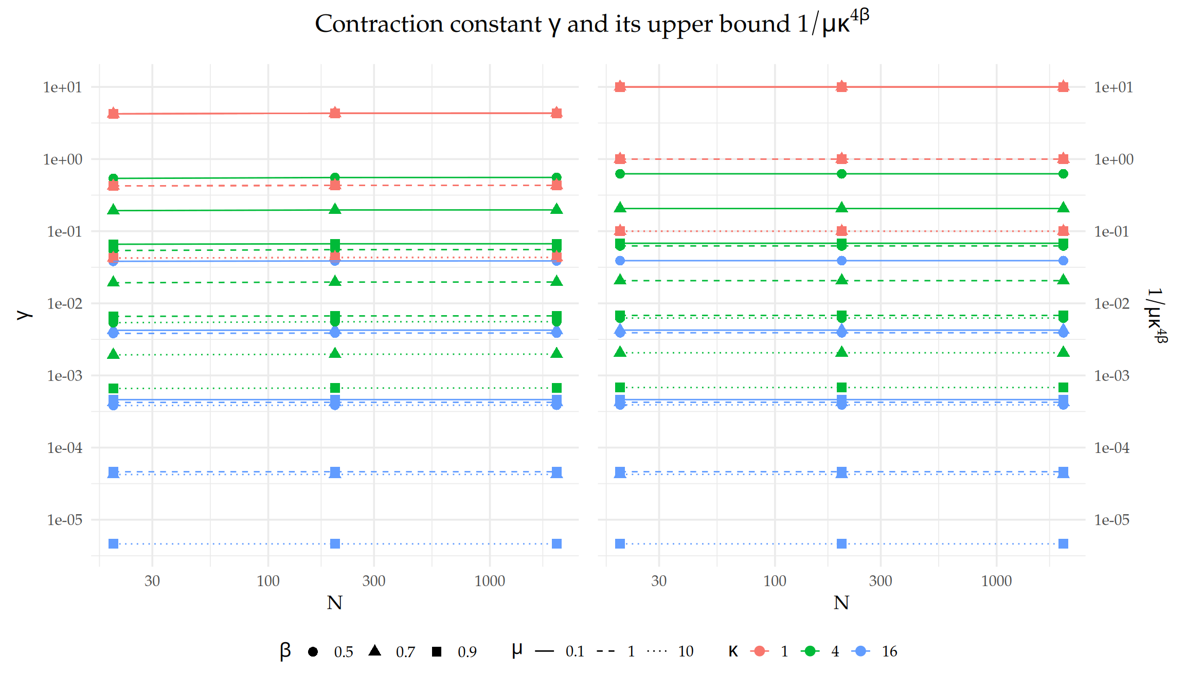
Figure 1: Comparison of the contraction constant \(\gamma = \tau^2\|\mathbf{T}\|_2/\mu\) and its theoretical upper bound \(1 / (\mu \kappa^{4 \beta})\) as functions of the sample size \(N\) for \(T = 2\). Different colors, shapes, and line types correspond to variations in \(\kappa\), \(\beta\), and \(\mu\), respectively. Both plots have their x- and y-axes on a \(\log_{10}\) scale, and they share the same y-axis limits for direct comparability.
1.11 References
We used R version 4.5.2 (R Core Team 2025) and the following R packages: akima v. 0.6.3.6 (Akima and Gebhardt 2025), expm v. 1.0.0 (Maechler, Dutang, and Goulet 2024), fmesher v. 0.5.0 (Lindgren 2025), gsignal v. 0.3.7 (Van Boxtel, G.J.M., et al. 2021), here v. 1.0.1 (Müller 2020), htmltools v. 0.5.8.1 (Cheng et al. 2024), INLA v. 25.11.22 (Rue, Martino, and Chopin 2009; Lindgren, Rue, and Lindström 2011; Martins et al. 2013; Lindgren and Rue 2015; De Coninck et al. 2016; Rue et al. 2017; Verbosio et al. 2017; Bakka et al. 2018; Kourounis, Fuchs, and Schenk 2018), inlabru v. 2.13.0 (Yuan et al. 2017; Bachl et al. 2019), knitr v. 1.50 (Xie 2014, 2015, 2025a), Matrix v. 1.7.3 (Bates, Maechler, and Jagan 2025), MetricGraph v. 1.5.0.9000 (Bolin, Simas, and Wallin 2023a, 2023b, 2024, 2025; Bolin et al. 2024), neuralnet v. 1.44.2 (Fritsch, Guenther, and Wright 2019), orthopolynom v. 1.0.6.1 (Novomestky 2022), patchwork v. 1.3.1 (Pedersen 2025), pbmcapply v. 1.5.1 (Kuang, Kong, and Napolitano 2022), plotly v. 4.11.0 (Sievert 2020), posterdown v. 1.0 (Thorne 2019), pracma v. 2.4.4 (Borchers 2023), qrcode v. 0.3.0 (Onkelinx and Teh 2024), RColorBrewer v. 1.1.3 (Neuwirth 2022), RefManageR v. 1.4.0 (McLean 2014, 2017), renv v. 1.1.5 (Ushey and Wickham 2025), reshape2 v. 1.4.4 (Wickham 2007), reticulate v. 1.44.1 (Ushey, Allaire, and Tang 2025), rmarkdown v. 2.30 (Xie, Allaire, and Grolemund 2018; Xie, Dervieux, and Riederer 2020; Allaire et al. 2025), rSPDE v. 2.5.1.9000 (Bolin and Kirchner 2020; Bolin and Simas 2023; Bolin, Simas, and Xiong 2024), RSpectra v. 0.16.2 (Qiu and Mei 2024), scales v. 1.4.0 (Wickham, Pedersen, and Seidel 2025), slackr v. 3.4.0 (Kaye et al. 2025), tidyverse v. 2.0.0 (Wickham et al. 2019), viridisLite v. 0.4.2 (Garnier et al. 2023), xaringan v. 0.31 (Xie 2025b), xaringanExtra v. 0.8.0 (Aden-Buie and Warkentin 2024), xaringanthemer v. 0.4.4 (Aden-Buie 2025).