Numerical approximation and optimal control of fractional diffusion equations on metric graphs

Lenin Rafael Riera Segura¹, David Bolin¹, Alexandre B. Simas¹

¹ Statistics Program, CEMSE, King Abdullah University of Science and Technology (KAUST), Thuwal, 23955-6900, Kingdom of Saudi Arabia

Introduction

We analyze and numerically approximate solutions to fractional diffusion equations on metric graphs of the form \[\begin{equation} \label{eq:maineqfirstpart} \tag{1} \left\{ \begin{aligned} \partial_t u(s,t) + L^{\alpha/2} u(s,t) &= f(s,t), \\ u(s,0) &= u_0(s), \end{aligned} \right. \end{equation}\] where $L = \kappa^2 \! - \! \Delta_\Gamma$ and $u(\cdot,t)$ satisfies the Kirchhoff vertex conditions \[\begin{equation} \label{eq:Kcondfirstpart} \tag{2} \textstyle\mathcal{K} = \left\{\phi\in C(\Gamma)\;\middle|\; \forall v\in \mathcal{V}:\; \sum_{e\in\mathcal{E}_v}\partial_e \phi(v)=0 \right\}. \end{equation}\] Here $\Gamma = (\mathcal{V},\mathcal{E})$ is a compact metric graph, $\kappa>0$, $\alpha\in(0,2]$ determines the smoothness of $u(\cdot,t)$, $\Delta_{\Gamma}$ is the so-called Kirchhoff–Laplacian. The fractional operator $L^{\alpha/2} : D(L^{\alpha/2}) \longmapsto L_2(\Gamma)$ is defined via \[\begin{equation} \label{lfractional} \textstyle \phi \longmapsto L^{\alpha/2}\phi = \sum_{j\in\mathbb{N}}\lambda_j^{\alpha/2}(\phi, e_j)_{L_2(\Gamma)}e_j, \end{equation}\] and $-L^{\alpha/2}$ generates $T(t)\phi = \sum_{j\in\mathbb{N}}e^{-\lambda^{\alpha/2}_jt}\left(\phi, e_j\right)_{L_2(\Gamma)}e_j$.

We interpret $\eqref{eq:maineqfirstpart}$ as an abstract Cauchy problem in $L_2(\Gamma)$, given by \[\begin{equation} \label{eq:cauchyproblem} \tag{3} \begin{cases} \partial_tu(t)+L^{\alpha/2}u(t)=f(t),\quad t\in (0, T),\\ u(0)=u_0\in D(L^{\alpha/2}). \end{cases} \end{equation}\]

Theorem 1. If $f\in L_2((0,T);L_2(\Gamma))$ and $u_0\in \dot{H}^{\alpha}(\Gamma)$, then $\eqref{eq:cauchyproblem}$ has a unique mild solution given by the variation of parameters formula \[\begin{equation} \label{eq:mildsolution} u(t) = T(t)u_0 + \int_0^t T(t-r)f(r)dr,\quad t\geq 0. \end{equation}\]

Numerical Approximation

Let $\kappa=1$. For all $\phi\in V_h$ and $k=0,\dots, N-1$, the discrete scheme computes $U_h^{\tau}\subset V_h$, which solves \[\begin{equation} \label{system:fully_discrete_scheme} \tag{4} \left\{ \begin{aligned} \langle\delta U_h^{k+1},\phi\rangle + \mathfrak{a}( U_h^{k+1},\phi) &= \langle f^{k+1},\phi\rangle, \\ U^0_h &= P_hu_0, \end{aligned} \right. \end{equation}\]

The corresponding strong form of $\eqref{system:fully_discrete_scheme}$ is given by \[\begin{align} \label{weak_form_m1} \tag{5} \textstyle (I_{V_h}+\tau L_h^{\alpha/2})U_h^{k+1} = U_h^{k}+\tau f^{k+1}. \end{align}\] By applying $L_h^{-\alpha/2}$ to $\eqref{weak_form_m1}$, replacing $L_h^{-\alpha/2}$ with the rational approximation $r_m(L_h^{-1})$ $=$ $p_\ell(L_h)^{-1}p_r(L_h)$, and using the partial-fraction expansion $p_r(x)/(p_r(x)+\tau p_\ell(x))$ $=$ $\sum_{k=1}^{m+1}a_k(x-p_k)^{-1}$, we obtain \[\begin{align} \tag{6} \label{weak_form_m4} \textstyle U_{h,m}^{k+1}= \left(\sum_{k=1}^{m+1}a_k(L_h-p_kI_{V_h})^{-1}\right) (U_{h,m}^{k}+\tau f^{k+1}), \end{align}\] or in matrix form, \[\begin{align} \label{thenumericalscheme} \textstyle\mathbf{U}_{k+1} = \mathbf{R}(\mathbf{C}\mathbf{U}_k+\tau \mathbf{F}_{k+1}),\quad \mathbf{R} = \sum_{k=1}^{m+1} a_k\left(\mathbf{L}-p_k\mathbf{C}\right)^{-1}. \end{align}\]

Theorem 2. Let $u$ be the solution to $\eqref{eq:maineqfirstpart}$ and $U^{\tau}_{h,m}\subset V_h$ solve the weak form of $\eqref{weak_form_m4}$. If $f\in L_\infty((0,T);L_2(\Gamma))$ and $u_0\in\dot{H}^{\alpha}(\Gamma)$, then

\[\begin{align} \label{finalfinalestfirstpart} {\left\|u-U_{h,m}^\tau\right\|}_{L_2(\Gamma\times(0,T))}\lesssim\tau+h^\alpha + h^{\alpha-2}e^{-2\pi\sqrt{(1-\alpha/2)m}}. \end{align}\]

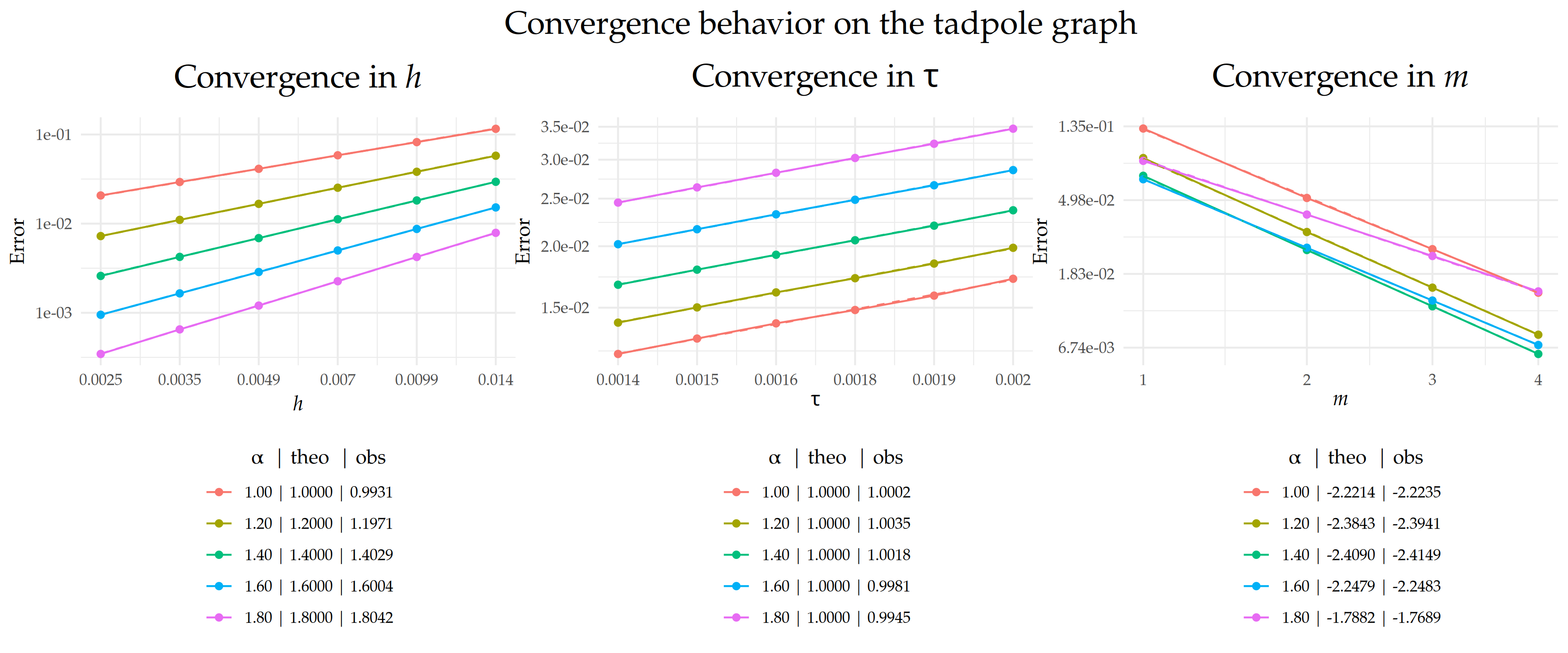
$Comparison between theoretical and observed convergence behavior for the error $\|u- U_{h,m}^\tau\|_{L_2(\Gamma\times(0,T))}$ with respect to $h$, $\tau$, and $m$, where $\Gamma$ is the tadpole graph. The left and center plots display the convergence rates in $h$ and $\tau$, respectively, on a $\text{log}_{10}$–$\text{log}_{10}$ scale, while the right plot shows the exponential decay in $m$ on a semi-$\text{log}_{e}$ scale, with $m$ plotted on a square-root scale. Dashed lines indicate the theoretical rates, and solid lines represent the observed error curves. The legend below each plot shows the value of $\alpha$ along with the corresponding theoretical ('theo'), and observed ('obs') rates for each case.$

Figure 1: Comparison between theoretical and observed convergence behavior for the error $\|u- U_{h,m}^\tau\|_{L_2(\Gamma\times(0,T))}$ with respect to $h$, $\tau$, and $m$, where $\Gamma$ is the tadpole graph. The left and center plots display the convergence rates in $h$ and $\tau$, respectively, on a $\text{log}_{10}$–$\text{log}_{10}$ scale, while the right plot shows the exponential decay in $m$ on a semi-$\text{log}_{e}$ scale, with $m$ plotted on a square-root scale. Dashed lines indicate the theoretical rates, and solid lines represent the observed error curves. The legend below each plot shows the value of $\alpha$ along with the corresponding theoretical (‘theo’), and observed (‘obs’) rates for each case.

Optimal Control Problem

Let $u_d$ be the desired state, $z$ denote the control variable, and $\mu>0$ a regularization parameter. We are concerned with the following PDE-constrained optimization problem: Find \[\begin{equation} \label{eq:min_pro} \tag{7} \min\; J(u, z)= \frac{1}{2} \int_0^T\left(\left\|u-u_d\right\|_{L_2(\Gamma)}^2+\mu\|z\|_{L_2(\Gamma)}^2\right) dt \end{equation}\] subject to the fractional diffusion equation $\eqref{eq:maineqfirstpart}$ with right-hand side $f+z$, where $u$ satisfies the Kirchhoff vertex conditions $\eqref{eq:Kcondfirstpart}$, and $z$ satisfies the control constraints \[\begin{align} \tag{9} \label{control_constraints} a(s,t)\leq z(s,t)\leq b(s,t)\;\mathrm{a.e.}\;(s,t)\in\Gamma \times(0, T). \end{align}\] Associated to $u = u(z)$, the adjoint state $p=p(z)$ solves \[\begin{equation} \tag{10} \label{eq:adjointeq} \left\{ \begin{aligned} \!-\partial_t p(s,t)\! + \! (\kappa^2 \! - \! \Delta_\Gamma)^{\alpha/2} p(s,t) &= \! u(s,t) \! - \! u_d(s,t),\\ p(s,T) &= \! 0. \end{aligned} \right. \end{equation}\]

The optimal control variable $\bar{z}$ is related to the optimal adjoint state $\bar{p}$ via the projection formula \[\begin{align} \tag{11} \label{proj_formula} \bar{z} = \min\left\{b ,\max\left\{a ,-\bar{p}/\mu \right\}\right\}. \end{align}\]

Theorem 3. Let $\bar{z}$ be the optimal control of problem $\eqref{eq:min_pro}$-$\eqref{control_constraints}$ and $\bar{Z}_{h,m}^\tau$ be the optimal discrete control. If $f,u_d\in L_\infty((0,T);L_2(\Gamma))$ and $u_0\in\dot{H}^{\alpha}(\Gamma)$, then

\[\begin{align} {\left\|\bar{z}- \bar{Z}_{h,m}^\tau\right\|}_{L_2(\Gamma\times(0,T))}\lesssim \tau+h^\alpha+ h^{\alpha-2}e^{-2\pi\sqrt{(1-\alpha/2)m}}. \end{align}\]

FBSM Algorithm

At a high level, FBSM follows these steps.

Initialization: Choose an initial approximation for $\bar{z}$.
State solve: Using $\bar{z}$, solve $\eqref{eq:maineqfirstpart}$ with RHS $f+\bar{z}$ to obtain $\bar{u}$.
Adjoint solve: Using $\bar{u}$, solve $\eqref{eq:adjointeq}$ to obtain $\bar{p}$.
Control update: Update $\bar{z}$ via the projection formula $\eqref{proj_formula}$.
Iteration: Repeat steps b - d until convergence.

The fully discrete and vectorized form is given by

Initialize $\mathbf{\bar{z}}$,
Compute $\mathbf{\bar{u}} = \mathbf{h} + \mathbf{S}_{\mathrm{F}}\mathbf{\hat{R}}(\mathbf{f}+\mathbf{M}\mathbf{\bar{z}})$,
Compute $\mathbf{\bar{p}} = \mathbf{S}_{\mathrm{B}}\mathbf{\hat{R}}(\mathbf{M}\mathbf{\bar{u}} - \mathbf{d})$,
Update $\mathbf{\bar{z}} = \max\{\mathbf{a}, \min\{\mathbf{b}, -\mathbf{\bar{p}}/\mu\}\}$,
Repeat 2 - 4 until convergence.

Let $\Pi(\mathbf{x}) := \max\{\mathbf{a}, \min\{\mathbf{b}, -\mathbf{x}/\mu\}\}$. Then the control update can be expressed as \[\begin{align*} \mathbf{\bar{z}} = \underbrace{\Pi(\mathbf{S}_{\mathrm{B}}\mathbf{\hat{R}}(\mathbf{M}(\mathbf{h} + \mathbf{S}_{\mathrm{F}}\mathbf{\hat{R}}(\mathbf{f}+\mathbf{M}\mathbf{\bar{z}})) - \mathbf{d}))}_{\mathfrak{T}(\mathbf{\bar{z}})}, \end{align*}\] which leads to the fixed-point formulation $\mathbf{\bar{z}}^{(n+1)} = \mathfrak{T}(\mathbf{\bar{z}}^{(n)})$.

Proposition 1. If $\mu\kappa^{2\alpha}>1$, then $\mathfrak{T}$ is a contraction and $(\mathbf{\bar{z}}^{(n)})_{n\in\mathbb{N}}$ converges to a unique fixed point $\mathbf{\bar{z}}^\star$, which uniquely determines the optimal state via $\mathbf{\bar{u}}^{\star} = \mathbf{h} + \mathbf{S}_{\mathrm{F}}\mathbf{\hat{R}}(\mathbf{f}+\mathbf{M}\mathbf{\bar{z}}^{\star})$.

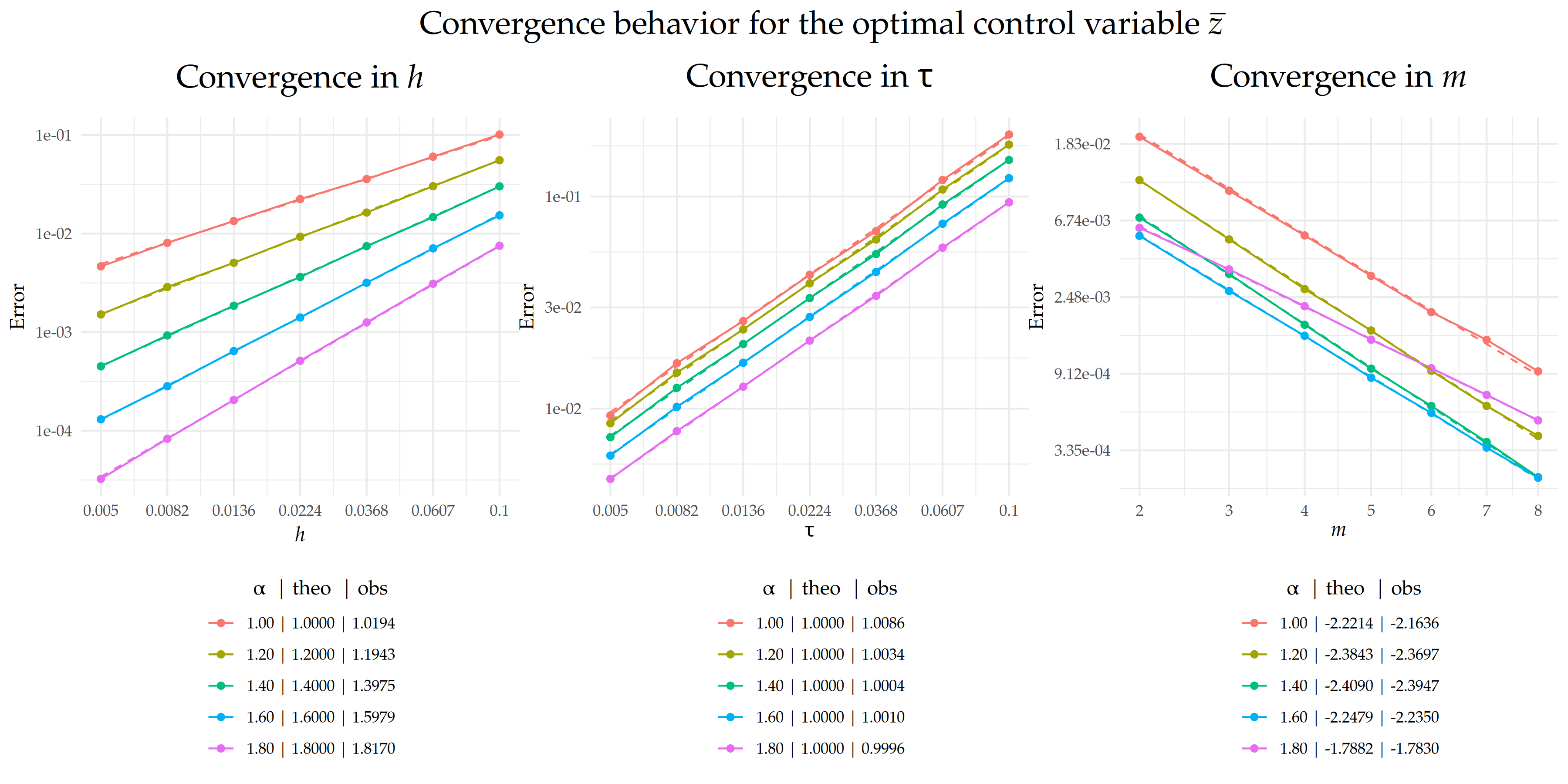
$Comparison between theoretical and observed convergence behavior for the error $\|\bar{z}- \bar{Z}_{h,m}^\tau\|_{L_2(\Gamma\times(0,T))}$ with respect to $h$, $\tau$, and $m$.$

Figure 2: Comparison between theoretical and observed convergence behavior for the error $\|\bar{z}- \bar{Z}_{h,m}^\tau\|_{L_2(\Gamma\times(0,T))}$ with respect to $h$, $\tau$, and $m$.

Figure 3: Visit https://leninrafaelrierasegura.github.io/NAFDEMG/ for more information.