This page shows a brief description of the contents of this website.

1 Contents

Contents: The current page.

2 Preliminaries

Preliminaries: This page shows
- how the finite element basis functions are constructed on a metric graph (see the Basis page for an additional illustration),
- how the eigenvalues and eigenfunctions of the shifted Kirchhoff–Laplacian $(\kappa^2-\Delta_\Gamma)$ operator are computed on the tadpole graph,
- and how to project onto a fine space-time mesh.

3 Results for the Numerical approximation of fractional diffusion equations on metric graphs paper

The illustration below was produced here.

Figure 1: Illustration of the system of basis functions $\{\varphi_j^e, \phi_v\}$ on the tadpole graph. Notice that the sets $\mathcal{N}_{v}$ are depicted in green and their corresponding basis functions are shown in red.

Functionality: This page shows

Experiment: This page shows
- how to construct an exact solution to the addressed problem for error analysis purposes.

Figure 2: Time evolution of the right-hand side function $f$.

Figure 3: Time evolution of the absolute difference between the exact and approximate solution.

Convergence in 𝘩: This page shows
- the convergence with respect to the spatial mesh size 𝘩.
Convergence in τ: This page shows
- the convergence with respect to the temporal mesh size τ.
Convergence in 𝑚: This page shows
- the convergence with respect to the order 𝑚 of the rational approximation.

Figure 1 shows the convergence results. For details on how these plots were generated, please refer to the hyperlinks above.

Metric graph

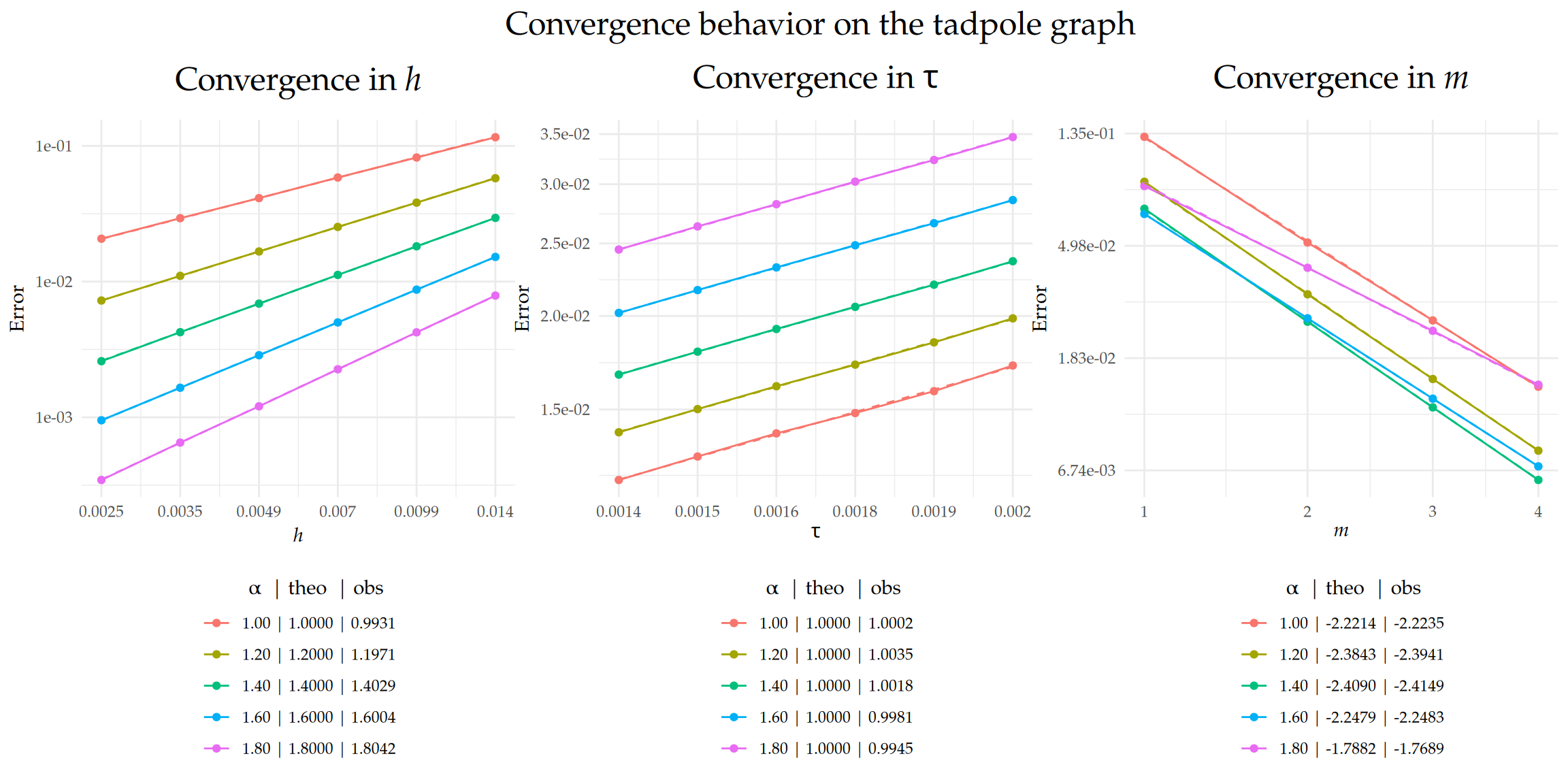
$Figure 4: Comparison of theoretical and observed convergence behavior for the $L_2(\Gamma\times(0,T))$-error with respect to $h$, $\tau$, and $m$. The left and center plots display the convergence rates in $h$ and $\tau$, respectively, on a $\text{log}_{10}$–$\text{log}_{10}$ scale, while the right plot shows the exponential decay in $m$ on a semi-$\text{log}_{e}$ scale, with $m$ plotted on a square-root scale. Dashed lines indicate the theoretical rates, and solid lines represent the observed error curves. The legend below each plot shows the value of $\alpha$ along with the corresponding theoretical ('theo'), and observed ('obs') rates for each case.$

Figure 4: Comparison of theoretical and observed convergence behavior for the $L_2(\Gamma\times(0,T))$-error with respect to $h$, $\tau$, and $m$. The left and center plots display the convergence rates in $h$ and $\tau$, respectively, on a $\text{log}_{10}$–$\text{log}_{10}$ scale, while the right plot shows the exponential decay in $m$ on a semi-$\text{log}_{e}$ scale, with $m$ plotted on a square-root scale. Dashed lines indicate the theoretical rates, and solid lines represent the observed error curves. The legend below each plot shows the value of $\alpha$ along with the corresponding theoretical (‘theo’), and observed (‘obs’) rates for each case.

Rectangle

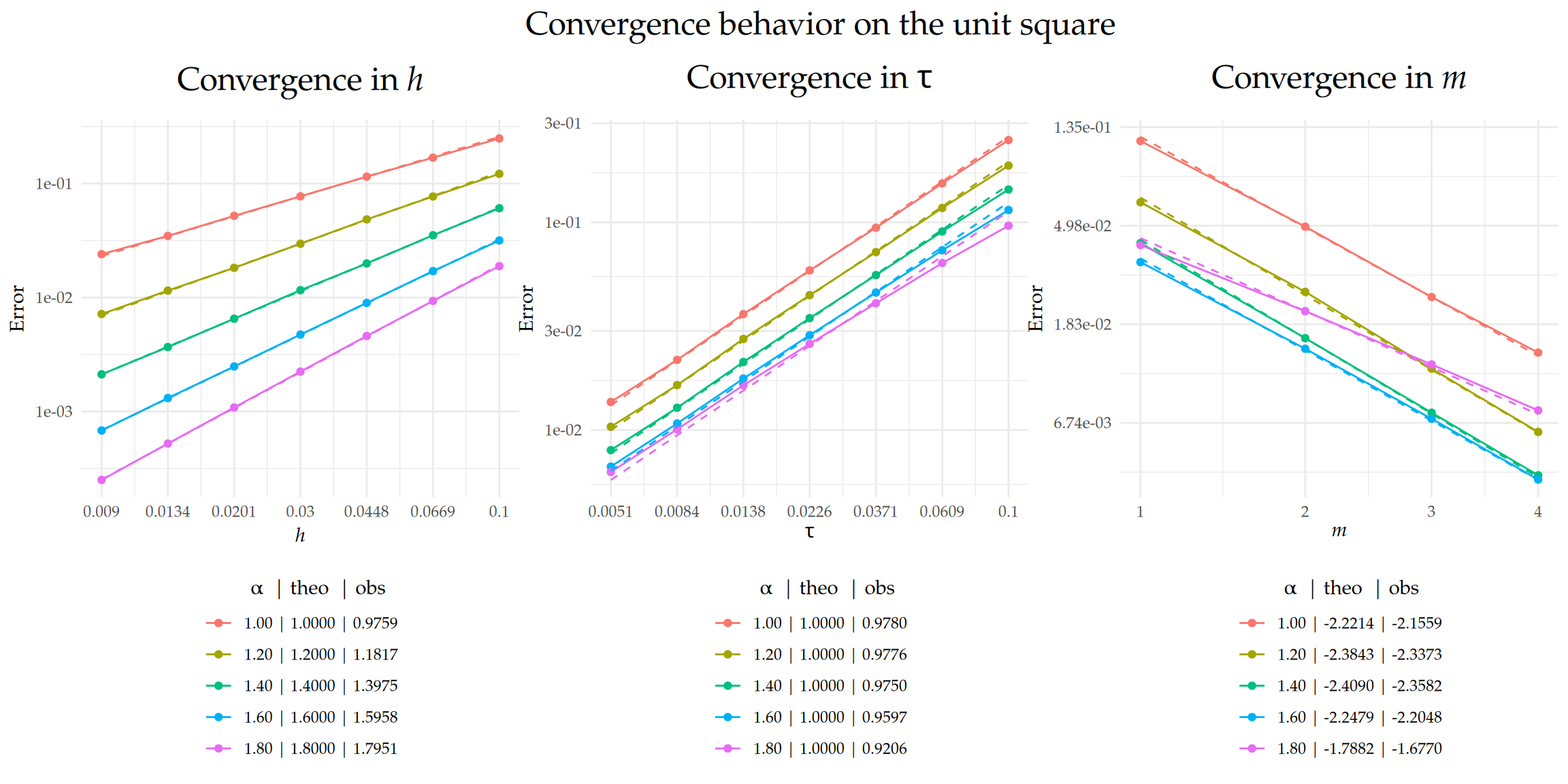
$Figure 5: Comparison of theoretical and observed convergence behavior for the $L_2(\Gamma\times(0,T))$-error with respect to $h$, $\tau$, and $m$. The left and center plots display the convergence rates in $h$ and $\tau$, respectively, on a $\text{log}_{10}$–$\text{log}_{10}$ scale, while the right plot shows the exponential decay in $m$ on a semi-$\text{log}_{e}$ scale, with $m$ plotted on a square-root scale. Dashed lines indicate the theoretical rates, and solid lines represent the observed error curves. The legend below each plot shows the value of $\alpha$ along with the corresponding theoretical ('theo'), and observed ('obs') rates for each case.$

Figure 5: Comparison of theoretical and observed convergence behavior for the $L_2(\Gamma\times(0,T))$-error with respect to $h$, $\tau$, and $m$. The left and center plots display the convergence rates in $h$ and $\tau$, respectively, on a $\text{log}_{10}$–$\text{log}_{10}$ scale, while the right plot shows the exponential decay in $m$ on a semi-$\text{log}_{e}$ scale, with $m$ plotted on a square-root scale. Dashed lines indicate the theoretical rates, and solid lines represent the observed error curves. The legend below each plot shows the value of $\alpha$ along with the corresponding theoretical (‘theo’), and observed (‘obs’) rates for each case.

Sphere

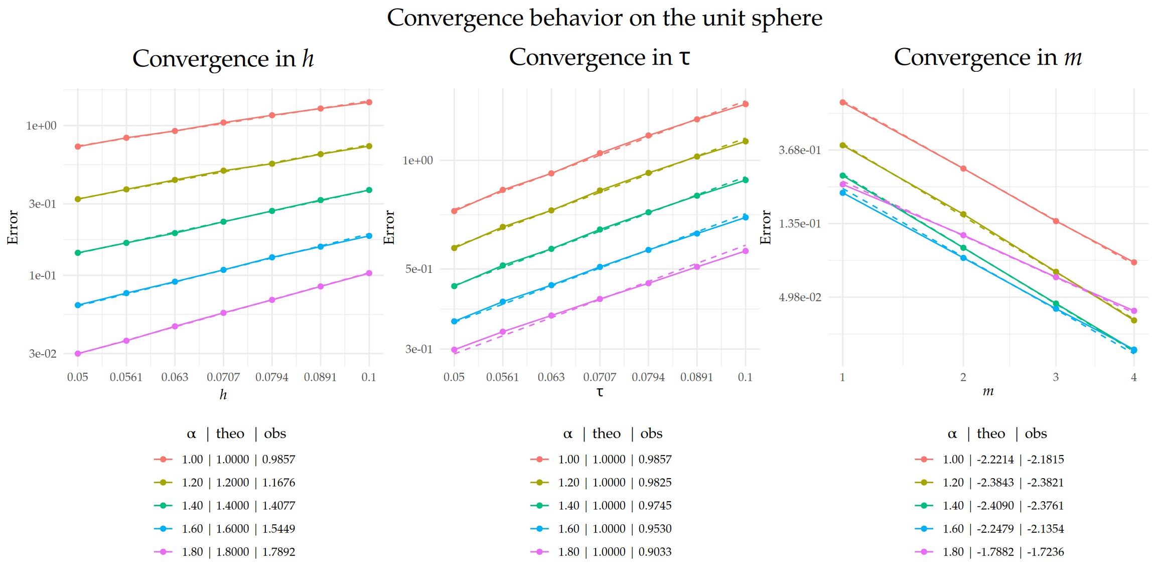
$Figure 6: Comparison of theoretical and observed convergence behavior for the $L_2(\Gamma\times(0,T))$-error with respect to $h$, $\tau$, and $m$. The left and center plots display the convergence rates in $h$ and $\tau$, respectively, on a $\text{log}_{10}$–$\text{log}_{10}$ scale, while the right plot shows the exponential decay in $m$ on a semi-$\text{log}_{e}$ scale, with $m$ plotted on a square-root scale. Dashed lines indicate the theoretical rates, and solid lines represent the observed error curves. The legend below each plot shows the value of $\alpha$ along with the corresponding theoretical ('theo'), and observed ('obs') rates for each case.$

Figure 6: Comparison of theoretical and observed convergence behavior for the $L_2(\Gamma\times(0,T))$-error with respect to $h$, $\tau$, and $m$. The left and center plots display the convergence rates in $h$ and $\tau$, respectively, on a $\text{log}_{10}$–$\text{log}_{10}$ scale, while the right plot shows the exponential decay in $m$ on a semi-$\text{log}_{e}$ scale, with $m$ plotted on a square-root scale. Dashed lines indicate the theoretical rates, and solid lines represent the observed error curves. The legend below each plot shows the value of $\alpha$ along with the corresponding theoretical (‘theo’), and observed (‘obs’) rates for each case.

4 Results for the Optimal control of fractional diffusion equations on metric graphs paper

Figure 7: Illustration of the basis function system $\{\psi^i_h\}_{i=1}^{N_h}$ on the hat-basis-functions graph (in black). Standard hat functions associated with internal edge nodes are shown in blue, while special vertex-centered functions are highlighted in red.

Control Functionality: This page shows

Optimal Control: This page shows
- how to construct an exact solution for the optimal control problem for error analysis purposes.

Convergence in 𝘩: This page shows
- the convergence with respect to the spatial mesh size 𝘩.

$Figure 8: Comparison of theoretical and observed convergence behavior for the $L_2(\Gamma\times(0,T))$-error with respect to $h$ on a $\text{log}_{10}$–$\text{log}_{10}$ scale. Dashed lines indicate the theoretical rates, and solid lines represent the observed error curves. The legend below each plot shows the value of $\alpha$ along with the corresponding theoretical ('theo'), and observed ('obs') rates for each case.$

Figure 8: Comparison of theoretical and observed convergence behavior for the $L_2(\Gamma\times(0,T))$-error with respect to $h$ on a $\text{log}_{10}$–$\text{log}_{10}$ scale. Dashed lines indicate the theoretical rates, and solid lines represent the observed error curves. The legend below each plot shows the value of $\alpha$ along with the corresponding theoretical (‘theo’), and observed (‘obs’) rates for each case.

Convergence in τ: This page shows
- the convergence with respect to the temporal mesh size τ.

$Figure 9: Comparison of theoretical and observed convergence behavior for the $L_2(\Gamma\times(0,T))$-error with respect to $\tau$ on a $\text{log}_{10}$–$\text{log}_{10}$ scale. Dashed lines indicate the theoretical rates, and solid lines represent the observed error curves. The legend below each plot shows the value of $\alpha$ along with the corresponding theoretical ('theo'), and observed ('obs') rates for each case.$

Figure 9: Comparison of theoretical and observed convergence behavior for the $L_2(\Gamma\times(0,T))$-error with respect to $\tau$ on a $\text{log}_{10}$–$\text{log}_{10}$ scale. Dashed lines indicate the theoretical rates, and solid lines represent the observed error curves. The legend below each plot shows the value of $\alpha$ along with the corresponding theoretical (‘theo’), and observed (‘obs’) rates for each case.

Convergence in 𝑚: This page shows
- the convergence with respect to the order 𝑚 of the rational approximation.

$Figure 10: Comparison of theoretical and observed convergence behavior for the $L_2(\Gamma\times(0,T))$-error with respect to $m$ on a semi-$\text{log}_{e}$ scale, with $m$ plotted on a square-root scale. Dashed lines indicate the theoretical rates, and solid lines represent the observed error curves. The legend below each plot shows the value of $\alpha$ along with the corresponding theoretical ('theo'), and observed ('obs') rates for each case.$

Figure 10: Comparison of theoretical and observed convergence behavior for the $L_2(\Gamma\times(0,T))$-error with respect to $m$ on a semi-$\text{log}_{e}$ scale, with $m$ plotted on a square-root scale. Dashed lines indicate the theoretical rates, and solid lines represent the observed error curves. The legend below each plot shows the value of $\alpha$ along with the corresponding theoretical (‘theo’), and observed (‘obs’) rates for each case.

The following figures show the convergence results for the optimal state and control variables. They contain the same information as the above plots, but are combined into two single figures for each variable.

$Figure 11: Comparison between theoretical and observed convergence behavior for the error $\|\bar{u}-\bar{U}_{h,m}^\tau\|_{L_2(\Gamma\times(0,T))}$ with respect to $h$, $\tau$, and $m$. The left and center plots display the convergence rates in $h$ and $\tau$, respectively, on a $\text{log}_{10}$–$\text{log}_{10}$ scale, while the right plot shows the exponential decay in $m$ on a semi-$\text{log}_{e}$ scale, with $m$ plotted on a square-root scale. Dashed lines indicate the theoretical rates, and solid lines represent the observed error curves. The legend below each plot shows the value of $\alpha$ along with the corresponding theoretical ('theo'), and observed ('obs') rates for each case.$

Figure 11: Comparison between theoretical and observed convergence behavior for the error $\|\bar{u}-\bar{U}_{h,m}^\tau\|_{L_2(\Gamma\times(0,T))}$ with respect to $h$, $\tau$, and $m$. The left and center plots display the convergence rates in $h$ and $\tau$, respectively, on a $\text{log}_{10}$–$\text{log}_{10}$ scale, while the right plot shows the exponential decay in $m$ on a semi-$\text{log}_{e}$ scale, with $m$ plotted on a square-root scale. Dashed lines indicate the theoretical rates, and solid lines represent the observed error curves. The legend below each plot shows the value of $\alpha$ along with the corresponding theoretical (‘theo’), and observed (‘obs’) rates for each case.

$Figure 12: Comparison between theoretical and observed convergence behavior for the error $\|\bar{z}- \bar{\mathcal{Z}}_{h,m}^\tau\|_{L_2(\Gamma\times(0,T))}$ with respect to $h$, $\tau$, and $m$. The left and center plots display the convergence rates in $h$ and $\tau$, respectively, on a $\text{log}_{10}$–$\text{log}_{10}$ scale, while the right plot shows the exponential decay in $m$ on a semi-$\text{log}_{e}$ scale, with $m$ plotted on a square-root scale. Dashed lines indicate the theoretical rates, and solid lines represent the observed error curves. The legend below each plot shows the value of $\alpha$ along with the corresponding theoretical ('theo'), and observed ('obs') rates for each case.$

Figure 12: Comparison between theoretical and observed convergence behavior for the error $\|\bar{z}- \bar{\mathcal{Z}}_{h,m}^\tau\|_{L_2(\Gamma\times(0,T))}$ with respect to $h$, $\tau$, and $m$. The left and center plots display the convergence rates in $h$ and $\tau$, respectively, on a $\text{log}_{10}$–$\text{log}_{10}$ scale, while the right plot shows the exponential decay in $m$ on a semi-$\text{log}_{e}$ scale, with $m$ plotted on a square-root scale. Dashed lines indicate the theoretical rates, and solid lines represent the observed error curves. The legend below each plot shows the value of $\alpha$ along with the corresponding theoretical (‘theo’), and observed (‘obs’) rates for each case.

The following illustration was produced here.

$Figure 13: Comparison of the contraction constant $\gamma = \tau^2\|\mathbf{T}\|_2/\mu$ and its theoretical upper bound $1 / (\mu \kappa^{4 \beta})$ as functions of the sample size $N$ for $T = 2$. Different colors, shapes, and line types correspond to variations in $\kappa$, $\beta$, and $\mu$, respectively. Both plots have their x- and y-axes on a $\log_{10}$ scale, and they share the same y-axis limits for direct comparability.$

Figure 13: Comparison of the contraction constant $\gamma = \tau^2\|\mathbf{T}\|_2/\mu$ and its theoretical upper bound $1 / (\mu \kappa^{4 \beta})$ as functions of the sample size $N$ for $T = 2$. Different colors, shapes, and line types correspond to variations in $\kappa$, $\beta$, and $\mu$, respectively. Both plots have their x- and y-axes on a $\log_{10}$ scale, and they share the same y-axis limits for direct comparability.

5 Poster

Poster: This page shows the poster presented at The KAUST 2025 Workshop on Statistics.

6 Presentation

Presentation: This page shows a presentation about the two papers.