Model properties (\(\nu\) fixed)

Go back to the About page. To see how the covariance function changes when \(\nu\) changes, go to model_properties2.html.

This vignette illustrates how our proposed approach allows for Gaussian processes with general smoothness and non-stationary covariance on any compact metric graph. Recall that these processes are defined as solutions to \[\begin{equation}\label{SPDE}\tag{SPDE} (\kappa^2 - \Delta_{\Gamma})^{\alpha/2}(\tau u) = \mathcal{W}, \quad \text{on $\Gamma$}, \end{equation}\] where \(\Delta_{\Gamma}\) is the so-called Kirchhoff–Laplacian, \(\tau(\cdot)\) and \(\kappa(\cdot)\) are spatially varying functions that control the marginal variance and practical correlation range, respectively, \(\alpha>1/2\) controls the smoothness, and \(\mathcal{W}\) is Gaussian white noise defined on a probability space \(\left(\Omega,\mathcal{F},\mathbb{P}\right)\).

Below we set some global options for all code chunks in this document.

# Set seed for reproducibility
set.seed(1982) 
# Set global options for all code chunks
knitr::opts_chunk$set(
  # Disable messages printed by R code chunks
  message = FALSE,    
  # Disable warnings printed by R code chunks
  warning = FALSE,    
  # Show R code within code chunks in output
  echo = TRUE,        
  # Include both R code and its results in output
  include = TRUE,     
  # Evaluate R code chunks
  eval = TRUE,       
  # Enable caching of R code chunks for faster rendering
  cache = FALSE,      
  # Align figures in the center of the output
  fig.align = "center",
  # Enable retina display for high-resolution figures
  retina = 2,
  # Show errors in the output instead of stopping rendering
  error = TRUE,
  # Do not collapse code and output into a single block
  collapse = FALSE
)
# Start the figure counter
fig_count <- 0
# Define the captioner function
captioner <- function(caption) {
  fig_count <<- fig_count + 1
  paste0("Figure ", fig_count, ": ", caption)
}
# Define the function to truncate a number to two decimal places
truncate_to_two <- function(x) {
  floor(x * 100) / 100
}

Below we load the necessary libraries and define the auxiliary functions.

library(rSPDE)
library(MetricGraph)

library(dplyr)
library(plotly)
library(scales)
library(patchwork)
library(tidyr)

library(here)
library(rmarkdown)
# Cite all loaded packages
library(grateful) 

Below we define function compute_pcr(), which computes the practical correlation. It receives the output of the rSPDE::spde.matern.operators() function (when evaluated on compatible parameters) and a threshold cor_threshold. Using the correlation matrix and the geodesic distance matrix, for each point in the mesh, it computes the practical correlation range as the minimum geodesic distance such that the correlation is below a given threshold cor_threshold (usually defined as 0.1). The function returns a vector with the practical correlation range for each point in the mesh.

---

Press the Show button below to reveal the code.

---

compute_pcr <- function(op, cor_threshold) {
  
  # Compute the covariance matrix
  cov_matrix <- op$covariance_mesh() 
  # Compute the correlation matrix
  cor_matrix <-cov2cor(cov_matrix)
  # Compute the geodesic distance matrix
  op$graph$compute_geodist_mesh() 
  # Extract the geodesic distance matrix
  dist_matrix <- op$graph$mesh$geo_dist 
  # Initialize the vector to store the practical correlation range
  pcr <- numeric(dim(cor_matrix)[1]) 
  
  process_row <- function(row_index) {
    # For each row_index, create an auxiliary matrix aux_mat with the correlation and geodesic distance
    aux_mat <- cbind(cor_matrix[row_index, ], dist_matrix[row_index, ]) 
    # Order the auxiliary matrix by the geodesic distance
    ordered_aux_mat <- aux_mat[order(aux_mat[, 2]), ] 
    # Filter the auxiliary ordered matrix by the correlation threshold
    filtered_aux_mat <- ordered_aux_mat[ordered_aux_mat[,1] < cor_threshold, ] 
    if (nrow(filtered_aux_mat) > 0) {
      # Return the minimum geodesic distance such that the correlation is below the threshold
      return(filtered_aux_mat[1, 2]) 
    } else {
      # If the condition is not satisfied, record the minimum correlation value and return an error message
      min <- min(aux_mat[, 1])
      stop(paste0("The condition cor_matrix[row_index, ] < cor_threshold is not satisfied for row_index = ", 
                  row_index, ". Increase cor_threshold. The minimum value of cor_matrix[row_index, ] is ",
                  min))
    }
  }
  
  pcr <- sapply(1:dim(cor_matrix)[1], process_row)
  
  return(pcr)
}

Below we build the MetricGraph package’s logo graph and plot the mesh.

# This is a function from MetricGraph package that returns a list of edges
edges <- logo_lines() 
# Create a new graph object
logo_graph <- metric_graph$new(edges = edges, perform_merges = TRUE) 
# Prune the vertices
#logo_graph$prune_vertices()
# Build the mesh
logo_graph$build_mesh(h = 0.05) 
# Extract the mesh locations in Euclidean coordinates
xypoints <- logo_graph$mesh$V
# Create a plot of the mesh
plot_mesh <- logo_graph$plot(mesh = TRUE) + 
  ggtitle("Mesh") + 
  theme_minimal() + 
  theme(text = element_text(family = "Palatino"))
print(plot_mesh)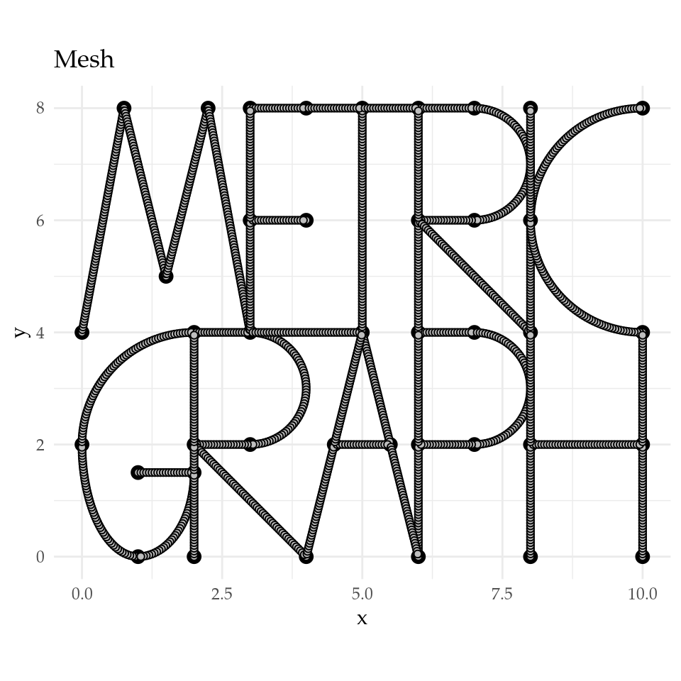

Figure 1: Mesh of the MetricGraph package’s logo.

Non-stationary features

Below we define \(\tau(\cdot)\) (model_for_tau) and \(\kappa(\cdot)\) (model_for_kappa) in \(\eqref{SPDE}\) as \(\tau(s) = \exp(0.05\cdot(x(s)-y(s)))\) and \(\kappa(s) = \exp(0.1\cdot(x(s)-y(s)))\), where \((x(s),y(s))\) are Euclidean coordinates on the plane. These choices make \(\tau(\cdot)\) and \(\kappa(\cdot)\) large in the bottom-right region of the MetricGraph package’s logo, as shown in Figure 2.

# Define an auxiliary variable
aux <- 0.1*(xypoints[,1] - xypoints[,2])
# Define the matrices B.tau and B.kappa
B.tau = cbind(0, 1, 0, 0.5*aux, 0)
B.kappa = cbind(0, 0, 1, 0, aux)
# Log-regression coefficients
theta <- c(0, 0, 1, 1) 
# Define the models for tau and kappa
model_for_tau <- exp(B.tau[,-1]%*%theta)
model_for_kappa <- exp(B.kappa[,-1]%*%theta)

Below we choose \(\alpha = 0.9\) and compute the covariance matrix, the practical correlation range, and the standard deviation.

# Choose alpha
nu = 0.4
alpha = nu + 1/2
# Compute the operator
op <- rSPDE::spde.matern.operators(graph = logo_graph,
                                      B.tau = B.tau,
                                      B.kappa =  B.kappa,
                                      parameterization = "spde",
                                      theta = theta,
                                      alpha = alpha)
# Compute the covariance matrix
est_cov_matrix <- op$covariance_mesh()
# Compute the practical correlation range
cor_threshold <- 0.1
est_range <- compute_pcr(op, cor_threshold)
# Compute the standard deviation
est_sigma <- sqrt(Matrix::diag(est_cov_matrix))

Below we plot the models for \(\tau(\cdot)\) and \(\kappa(\cdot)\), the practical correlation range, and the standard deviation. The blue, red, and green points represent the locations \(s_1\), \(s_2\), and \(s_3\), respectively.

---

Press the Show button below to reveal the code.

---

# Choose three points
point1 <- c(0.5670, 7.0243)
point2 <- c(0.03971546, 2.39628)
point3 <- c(10, 3)
# Find the indices of the three points
m1 <- which.min((xypoints[,1]-point1[1])^2 + (xypoints[,2]-point1[2])^2)
m2 <- which.min((xypoints[,1]-point2[1])^2 + (xypoints[,2]-point2[2])^2)
m3 <- which.min((xypoints[,1]-point3[1])^2 + (xypoints[,2]-point3[2])^2)
# Create a plot of the model for tau
TAU <- logo_graph$plot_function(X = model_for_tau, vertex_size = 0, plotly = FALSE) +
  ggtitle("Model for tau") +
  theme_minimal() +
  theme(text = element_text(family = "Palatino"))
# Create a plot of the model for kappa
KAPPA <- logo_graph$plot_function(X = model_for_kappa, vertex_size = 0, plotly = FALSE) +
  ggtitle("Model for kappa") +
  theme_minimal() +
  theme(text = element_text(family = "Palatino"))
# Create a plot for the practical correlation range
r1 <- logo_graph$plot_function(X = est_range, vertex_size = 0) +
  ggtitle("Practical correlation range") +
  theme_minimal() +
  theme(text = element_text(family = "Palatino")) +
  annotate("point", x = xypoints[m1,1], y = xypoints[m1,2], size = 1, color = "blue") +
  annotate("point", x = xypoints[m2,1], y = xypoints[m2,2], size = 1, color = "red") +
  annotate("point", x = xypoints[m3,1], y = xypoints[m3,2], size = 1, color = "darkgreen") +
  annotate("text", x = xypoints[m1,1] + 0.1, y = xypoints[m1,2] - 0.4, label = "s[1]", parse = TRUE, size = 3, hjust = 0, color = "black") +
  annotate("text", x = xypoints[m2,1] + 0.4, y = xypoints[m2,2], label = "s[2]", parse = TRUE, size = 3, hjust = 0, color = "black") +
  annotate("text", x = xypoints[m3,1] - 0.8, y = xypoints[m3,2], label = "s[3]", parse = TRUE, size = 3, hjust = 0, color = "black")
# Create a plot for the standard deviation
s1 <- logo_graph$plot_function(X = est_sigma, vertex_size = 0) +
  ggtitle("Standard deviation") +
  theme_minimal() +
  theme(text = element_text(family = "Palatino")) +
  annotate("point", x = xypoints[m1,1], y = xypoints[m1,2], size = 1, color = "blue") +
  annotate("point", x = xypoints[m2,1], y = xypoints[m2,2], size = 1, color = "red") +
  annotate("point", x = xypoints[m3,1], y = xypoints[m3,2], size = 1, color = "darkgreen") +
  annotate("text", x = xypoints[m1,1] + 0.1, y = xypoints[m1,2] - 0.4, label = "s[1]", parse = TRUE, size = 3, hjust = 0, color = "black") +
  annotate("text", x = xypoints[m2,1] + 0.4, y = xypoints[m2,2], label = "s[2]", parse = TRUE, size = 3, hjust = 0, color = "black") +
  annotate("text", x = xypoints[m3,1] - 0.8, y = xypoints[m3,2], label = "s[3]", parse = TRUE, size = 3, hjust = 0, color = "black")
# Combine the four plots
four_plots <- (TAU + KAPPA) / (s1 + r1)
# Save the combined plot
ggsave(here("data_files/four_plots.png"), plot = four_plots, width = 9.22, height = 7.05, dpi = 300)
# Print the combined plot
print(four_plots)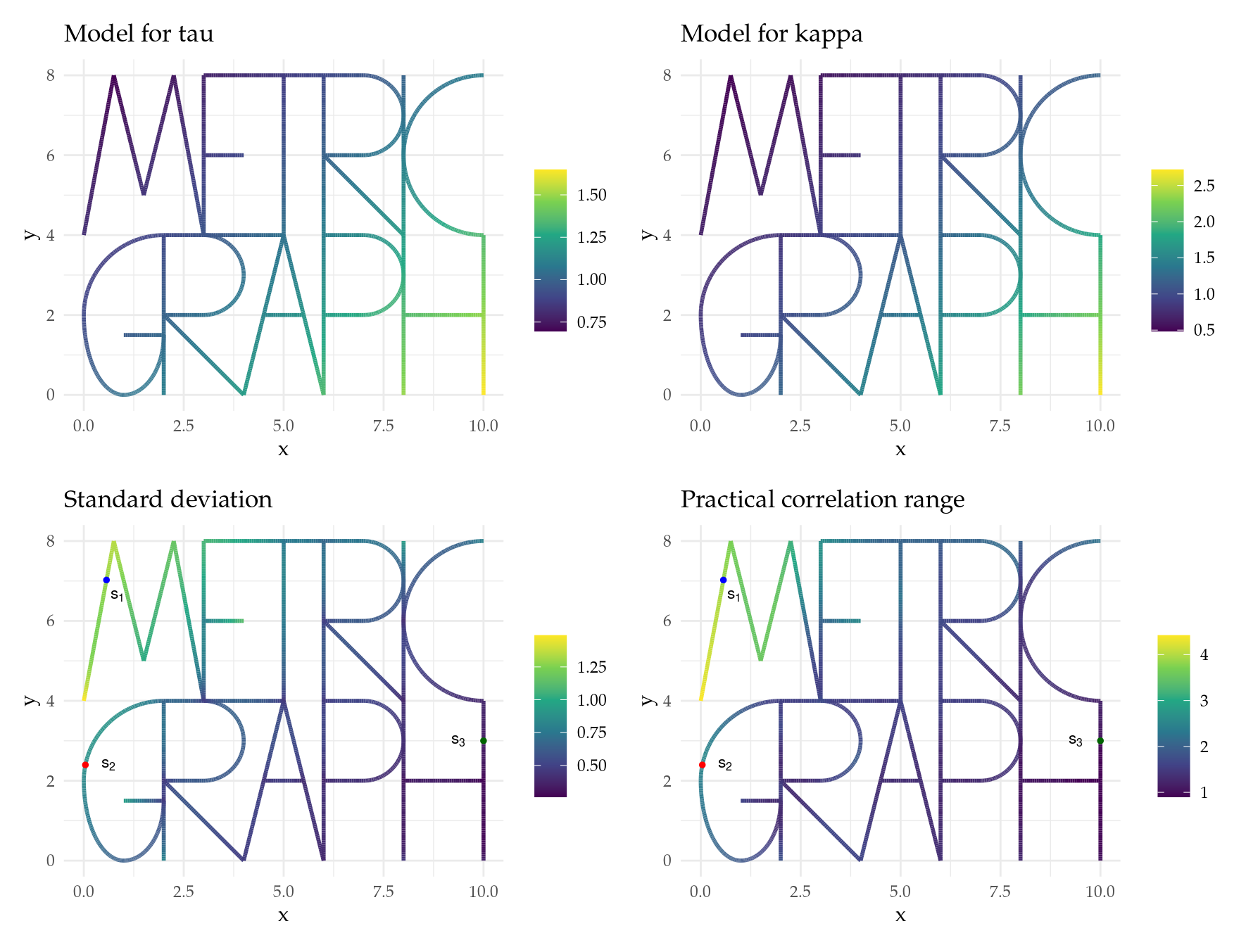

Figure 2: Top row: Non-stationary models for \(\tau(\cdot)\) and \(\kappa(\cdot)\). Bottom row: Non-stationary standard deviation and practical correlation range on the MetricGraph package’s logo.

Covariance plots

Below we plot the covariance functions \(r_i(\cdot)=\text{Cov}(u(s_i),u(\cdot))\), \(i=1,2,3\), for three locations with different standard deviations and practical correlation ranges on the MetricGraph package’s logo.

---

Press the Show button below to reveal the code.

---

# Create a plot for the covariance between point1 and all other points
c1 <- logo_graph$plot_function(X = est_cov_matrix[m1, ], vertex_size = 0) +
  ggtitle(latex2exp::TeX("$r_1$")) +
  theme_minimal() +
  theme(text = element_text(family = "Palatino"),
        plot.title = element_text(size = 12)) +
  annotate("point", x = xypoints[m1,1], y = xypoints[m1,2], size = 1, color = "blue") +
  annotate("text", x = xypoints[m1,1] + 0.1, y = xypoints[m1,2] - 0.4, label = "s[1]", parse = TRUE, size = 3, hjust = 0, color = "black")
# Create a plot for the covariance between point2 and all other points
c2 <- logo_graph$plot_function(X = est_cov_matrix[m2, ], vertex_size = 0) +
  ggtitle(latex2exp::TeX("$r_2$")) +
  theme_minimal() +
  theme(text = element_text(family = "Palatino"),
        plot.title = element_text(size = 12)) +
  annotate("point", x = xypoints[m2,1], y = xypoints[m2,2], size = 1, color = "red") +
  annotate("text", x = xypoints[m2,1] + 0.4, y = xypoints[m2,2], label = "s[2]", parse = TRUE, size = 3, hjust = 0, color = "black")
# Create a plot for the covariance between point3 and all other points
c3 <- logo_graph$plot_function(X = est_cov_matrix[m3, ], vertex_size = 0) +
  ggtitle(latex2exp::TeX("$r_3$")) +
  theme_minimal() +
  theme(text = element_text(family = "Palatino"),
        plot.title = element_text(size = 12)) +
  annotate("point", x = xypoints[m3,1], y = xypoints[m3,2], size = 1, color = "darkgreen") +
  annotate("text", x = xypoints[m3,1] - 0.8, y = xypoints[m3,2], label = "s[3]", parse = TRUE, size = 3, hjust = 0, color = "black")
# Combine the three plots
cs <- c1 + c2 + c3
# Save the combined plot
ggsave(here("data_files/cov_plots_diff_loc.png"), plot = cs, width = 13.83, height = 4.5, dpi = 300)
# Print the combined plot
print(cs)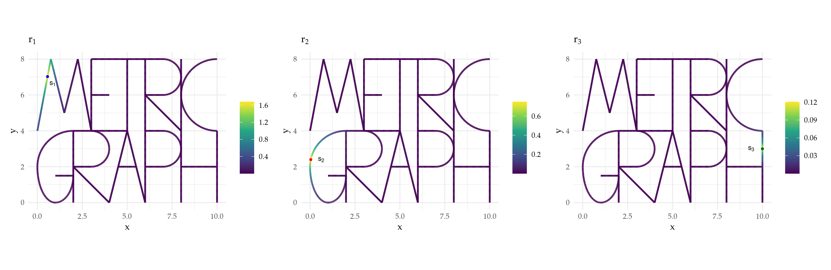

Figure 3: Example of covariance functions \(r_i(\cdot)\), \(i=1,2,3\) for three locations with different standard deviations and practical correlation ranges on the MetricGraph package’s logo.

Below we show 3D plots of the covariance functions \(r_i(\cdot)\), \(i=1,2,3\), for three locations with different standard deviations and practical correlation ranges on the MetricGraph package’s logo. The practical correlation range \(\rho(s_i)\) and the standard deviation \(\sigma(s_i)\) are also shown for each location \(s_i\).

---

Press the Show button below to reveal the code.

---

p1 <- logo_graph$plot_function(X = est_cov_matrix[m1, ], vertex_size = 1, plotly = TRUE, edge_color = "black", edge_width = 3, line_color = "blue", line_width = 3)
p2 <- logo_graph$plot_function(X = est_cov_matrix[m2, ], vertex_size = 1, plotly = TRUE, edge_color = "black", edge_width = 3, line_color = "red", line_width = 3, p = p1)
p3 <- logo_graph$plot_function(X = est_cov_matrix[m3, ], vertex_size = 1, plotly = TRUE, edge_color = "black", edge_width = 3, line_color = "darkgreen", line_width = 3, p = p2)
p <- p3 %>%
  config(mathjax = 'cdn') %>%
  layout(font = list(family = "Palatino"),
         showlegend = FALSE,
         scene = list(
           aspectratio = list(x = 1.8, y = 1.8, z = 1.8),
           camera = list(
      eye = list(x = 3, y = 2, z = 0.5),  # Adjust the viewpoint
      center = list(x = 0, y = 0, z = 0)),     # Focus point
           annotations = list(
             list(
               x = 3, y = 4, z = 1.4,
               text = TeX("\\rho(s_i)"),
               textangle = 0, ax = 60, ay = 0,
               font = list(color = "black", size = 16),
               arrowcolor = "white", arrowsize = 1, arrowwidth = 0.1, arrowhead = 1),
             list(
               x = 3, y = 4, z = 1.23,
               text = TeX(paste0("\\bullet\\mbox{ ", truncate_to_two(est_range[m1]), "}")),
               textangle = 0, ax = 60, ay = 0,
               font = list(color = "blue", size = 16),
               arrowcolor = "white", arrowsize = 1, arrowwidth = 0.1, arrowhead = 1),
             list(
               x = 3, y = 4, z = 1.11,
               text = TeX(paste0("\\bullet\\mbox{ ", truncate_to_two(est_range[m2]), "}")),
               textangle = 0, ax = 60, ay = 0,
               font = list(color = "red", size = 16),
               arrowcolor = "white", arrowsize = 1, arrowwidth = 0.1, arrowhead = 1),
             list(
               x = 3, y = 4, z = 0.99,
               text = TeX(paste0("\\bullet\\mbox{ ", truncate_to_two(est_range[m3]), "}")),
               textangle = 0, ax = 60, ay = 0,
               font = list(color = "darkgreen", size = 16),
               arrowcolor = "white", arrowsize = 1, arrowwidth = 0.1, arrowhead = 1),
             list(
               x = 3, y = 6, z = 1.4,
               text = TeX("\\sigma(s_i)"),
               textangle = 0, ax = 60, ay = 0,
               font = list(color = "black", size = 16),
               arrowcolor = "white", arrowsize = 1, arrowwidth = 0.1, arrowhead = 1),
             list(
               x = 3, y = 6, z = 1.23,
               text = TeX(paste0("\\bullet\\mbox{ ", truncate_to_two(est_sigma[m1]), "}")),
               textangle = 0, ax = 60, ay = 0,
               font = list(color = "blue", size = 16),
               arrowcolor = "white", arrowsize = 1, arrowwidth = 0.1, arrowhead = 1),
             list(
               x = 3, y = 6, z = 1.11,
               text = TeX(paste0("\\bullet\\mbox{ ", truncate_to_two(est_sigma[m2]), "}")),
               textangle = 0, ax = 60, ay = 0,
               font = list(color = "red", size = 16),
               arrowcolor = "white", arrowsize = 1, arrowwidth = 0.1, arrowhead = 1),
             list(
               x = 3, y = 6, z = 0.99,
               text = TeX(paste0("\\bullet\\mbox{ ", truncate_to_two(est_sigma[m3]), "}")),
               textangle = 0, ax = 60, ay = 0,
               font = list(color = "darkgreen", size = 16),
               arrowcolor = "white", arrowsize = 1, arrowwidth = 0.1, arrowhead = 1),
             list(
               x = 3, y = 8, z = 1.4,
               text = TeX("\\alpha"),
               textangle = 0, ax = 60, ay = 0,
               font = list(color = "black", size = 16),
               arrowcolor = "white", arrowsize = 1, arrowwidth = 0.1, arrowhead = 1),
             list(
               x = 3, y = 8, z = 1.23,
               text = TeX(paste0("\\bullet\\mbox{ ", alpha, "}")),
               textangle = 0, ax = 60, ay = 0,
               font = list(color = "black", size = 16),
               arrowcolor = "white", arrowsize = 1, arrowwidth = 0.1, arrowhead = 1),
             list(
               x = 8.5, y = 0.5, z = 0,
               text = TeX("s_1"),
               textangle = 0, ax = 0, ay = 15,
               font = list(color = "black", size = 16),
               arrowcolor = "white", arrowsize = 1, arrowwidth = 0.1, arrowhead = 1),
             list(
               x = 2.5, y = 0, z = 0,
               text = TeX("s_2"),
               textangle = 0, ax = 0, ay = 15,
               font = list(color = "black", size = 16),
               arrowcolor = "white", arrowsize = 1, arrowwidth = 0.1, arrowhead = 1),
             list(
               x = 3, y = 10, z = 0,
               text = TeX("s_3"),
               textangle = 0, ax = 0, ay = 15,
               font = list(color = "black", size = 16),
               arrowcolor = "white", arrowsize = 1, arrowwidth = 0.1, arrowhead = 1),
             list(
               x = xypoints[m1, 2], y = xypoints[m1, 1], z = max(est_cov_matrix[m1, ]) + 0.2,
               text = TeX("r_1(\\cdot)"),
               textangle = 0, ax = 0, ay = 15,
               font = list(color = "blue", size = 16),
               arrowcolor = "white", arrowsize = 1, arrowwidth = 0.1, arrowhead = 1),
             list(
               x = xypoints[m2, 2], y = xypoints[m2, 1], z = max(est_cov_matrix[m2, ]) + 0.2,
               text = TeX("r_2(\\cdot)"),
               textangle = 0, ax = 0, ay = 15,
               font = list(color = "red", size = 16),
               arrowcolor = "white", arrowsize = 1, arrowwidth = 0.1, arrowhead = 1),
             list(
               x = xypoints[m3, 2], y = xypoints[m3, 1], z = max(est_cov_matrix[m3, ]) + 0.2,
               text = TeX("r_3(\\cdot)"),
               textangle = 0, ax = 0, ay = 15,
               font = list(color = "darkgreen", size = 16),
               arrowcolor = "white", arrowsize = 1, arrowwidth = 0.1, arrowhead = 1)))) %>%
  add_trace(x = xypoints[m1, 2], y = xypoints[m1, 1], z = 0, mode = "markers", type = "scatter3d",
            marker = list(size = 4, color = "blue", symbol = 104)) %>%
  add_trace(x = xypoints[m2, 2], y = xypoints[m2, 1], z = 0, mode = "markers", type = "scatter3d",
            marker = list(size = 4, color = "red", symbol = 104)) %>%
  add_trace(x = xypoints[m3, 2], y = xypoints[m3, 1], z = 0, mode = "markers", type = "scatter3d",
            marker = list(size = 4, color = "darkgreen", symbol = 104))
# Save the 3D plot
save(p, file = here("data_files/3d_cov_plots_diff_loc.RData"))

# Print the 3D plot
p

Figure 4: Example of covariance functions \(r_i(\cdot)\), \(i=1,2,3\) for three locations with different standard deviations and practical correlation ranges on the MetricGraph package’s logo.

Below we simulate the non-stationary field and plot the graph and the non-stationary field.

---

Press the Show button below to reveal the code.

---

# Simulate the non-stationary field
u_non_stat <- simulate(op)
# Plot the graph
plot_graph <- logo_graph$plot(vertex_size = 1, vertex_color = "blue") +
  ggtitle(latex2exp::TeX("MetricGraph package's logo")) +
  theme_minimal() +
  theme(text = element_text(family = "Palatino"))
# Plot the non-stationary field
plot_sim <- logo_graph$plot_function(X = u_non_stat, vertex_size = 0) +
  ggtitle("Simulated non-stationary process") +
  theme_minimal() +
  theme(text = element_text(family = "Palatino"))
# Combine the two plots
graph_plus_sim <- plot_graph + plot_sim
# Save the combined plot
ggsave(here("data_files/graph_plus_sim.png"), plot = graph_plus_sim, width = 9.22, height = 4.01, dpi = 300)
# Print the combined plot
print(graph_plus_sim)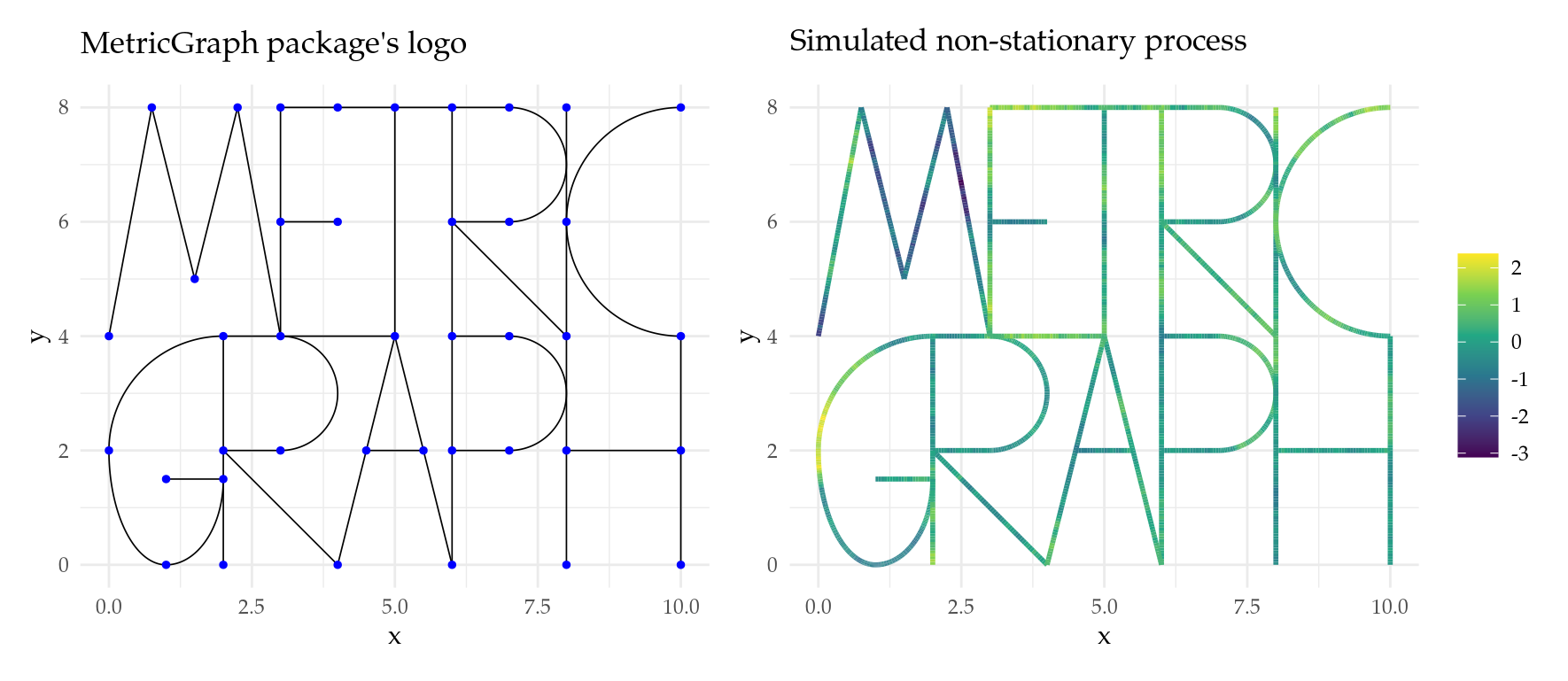

Figure 5: MetricGraph package’s logo and a simulated non-stationary process on it.

Here a list of the packages used in this document.

cite_packages(output = "paragraph", out.dir = ".")

We used R version 4.4.1 (R Core Team 2024a) and the following R packages: cowplot v. 1.1.3 (Wilke 2024), ggmap v. 4.0.0.900 (Kahle and Wickham 2013), ggpubr v. 0.6.0 (Kassambara 2023), ggtext v. 0.1.2 (Wilke and Wiernik 2022), grid v. 4.4.1 (R Core Team 2024b), here v. 1.0.1 (Müller 2020), htmltools v. 0.5.8.1 (Cheng et al. 2024), INLA v. 24.12.11 (Rue, Martino, and Chopin 2009; Lindgren, Rue, and Lindström 2011; Martins et al. 2013; Lindgren and Rue 2015; De Coninck et al. 2016; Rue et al. 2017; Verbosio et al. 2017; Bakka et al. 2018; Kourounis, Fuchs, and Schenk 2018), inlabru v. 2.12.0.9002 (Yuan et al. 2017; Bachl et al. 2019), knitr v. 1.48 (Xie 2014, 2015, 2024), latex2exp v. 0.9.6 (Meschiari 2022), Matrix v. 1.6.5 (Bates, Maechler, and Jagan 2024), MetricGraph v. 1.4.0.9000 (Bolin, Simas, and Wallin 2023b, 2023a, 2023c, 2024; Bolin et al. 2024), OpenStreetMap v. 0.4.0 (Fellows and JMapViewer library by Jan Peter Stotz 2023), osmdata v. 0.2.5 (Mark Padgham et al. 2017), patchwork v. 1.2.0 (Pedersen 2024), plotly v. 4.10.4 (Sievert 2020), plotrix v. 3.8.4 (J 2006), reshape2 v. 1.4.4 (Wickham 2007), rmarkdown v. 2.28 (Xie, Allaire, and Grolemund 2018; Xie, Dervieux, and Riederer 2020; Allaire et al. 2024), rSPDE v. 2.4.0.9000 (Bolin and Kirchner 2020; Bolin and Simas 2023; Bolin, Simas, and Xiong 2024), scales v. 1.3.0 (Wickham, Pedersen, and Seidel 2023), sf v. 1.0.19 (E. Pebesma 2018; E. Pebesma and Bivand 2023), sp v. 2.1.4 (E. J. Pebesma and Bivand 2005; Bivand, Pebesma, and Gomez-Rubio 2013), tidyverse v. 2.0.0 (Wickham et al. 2019), viridis v. 0.6.4 (Garnier et al. 2023), xaringanExtra v. 0.8.0 (Aden-Buie and Warkentin 2024).

Aden-Buie, Garrick, and Matthew T. Warkentin. 2024. xaringanExtra: Extras and Extensions for “xaringan” Slides. https://CRAN.R-project.org/package=xaringanExtra.

Allaire, JJ, Yihui Xie, Christophe Dervieux, Jonathan McPherson, Javier Luraschi, Kevin Ushey, Aron Atkins, et al. 2024. rmarkdown: Dynamic Documents for r. https://github.com/rstudio/rmarkdown.

Bachl, Fabian E., Finn Lindgren, David L. Borchers, and Janine B. Illian. 2019. “inlabru: An R Package for Bayesian Spatial Modelling from Ecological Survey Data.” Methods in Ecology and Evolution 10: 760–66. https://doi.org/10.1111/2041-210X.13168.

Bakka, Haakon, Håvard Rue, Geir-Arne Fuglstad, Andrea I. Riebler, David Bolin, Janine Illian, Elias Krainski, Daniel P. Simpson, and Finn K. Lindgren. 2018. “Spatial Modelling with INLA: A Review.” WIRES (Invited Extended Review) xx (Feb): xx–. http://arxiv.org/abs/1802.06350.

Bates, Douglas, Martin Maechler, and Mikael Jagan. 2024. Matrix: Sparse and Dense Matrix Classes and Methods. https://CRAN.R-project.org/package=Matrix.

Bivand, Roger S., Edzer Pebesma, and Virgilio Gomez-Rubio. 2013. Applied Spatial Data Analysis with R, Second Edition. Springer, NY. https://asdar-book.org/.

Bolin, David, and Kristin Kirchner. 2020. “The Rational SPDE Approach for Gaussian Random Fields with General Smoothness.” Journal of Computational and Graphical Statistics 29 (2): 274–85. https://doi.org/10.1080/10618600.2019.1665537.

Bolin, David, Mihály Kovács, Vivek Kumar, and Alexandre B. Simas. 2024. “Regularity and Numerical Approximation of Fractional Elliptic Differential Equations on Compact Metric Graphs.” Mathematics of Computation 93 (349): 2439–72. https://doi.org/10.1090/mcom/3929.

Bolin, David, and Alexandre B. Simas. 2023. rSPDE: Rational Approximations of Fractional Stochastic Partial Differential Equations. https://CRAN.R-project.org/package=rSPDE.

Bolin, David, Alexandre B. Simas, and Jonas Wallin. 2023a. “Markov Properties of Gaussian Random Fields on Compact Metric Graphs.” arXiv Preprint arXiv:2304.03190. https://doi.org/10.48550/arXiv.2304.03190.

———. 2023b. MetricGraph: Random Fields on Metric Graphs. https://CRAN.R-project.org/package=MetricGraph.

———. 2023c. “Statistical Inference for Gaussian Whittle-Matérn Fields on Metric Graphs.” arXiv Preprint arXiv:2304.10372. https://doi.org/10.48550/arXiv.2304.10372.

———. 2024. “Gaussian Whittle-Matérn Fields on Metric Graphs.” Bernoulli 30 (2): 1611–39. https://doi.org/10.3150/23-BEJ1647.

Bolin, David, Alexandre B. Simas, and Zhen Xiong. 2024. “Covariance-Based Rational Approximations of Fractional SPDEs for Computationally Efficient Bayesian Inference.” Journal of Computational and Graphical Statistics 33 (1): 64–74. https://doi.org/10.1080/10618600.2023.2231051.

Cheng, Joe, Carson Sievert, Barret Schloerke, Winston Chang, Yihui Xie, and Jeff Allen. 2024. htmltools: Tools for HTML. https://CRAN.R-project.org/package=htmltools.

De Coninck, Arne, Bernard De Baets, Drosos Kourounis, Fabio Verbosio, Olaf Schenk, Steven Maenhout, and Jan Fostier. 2016. “Needles: Toward Large-Scale Genomic Prediction with Marker-by-Environment Interaction.” Genetics 203 (1): 543–55. https://doi.org/10.1534/genetics.115.179887.

Fellows, Ian, and using the JMapViewer library by Jan Peter Stotz. 2023. OpenStreetMap: Access to Open Street Map Raster Images. https://CRAN.R-project.org/package=OpenStreetMap.

Garnier, Simon, Ross, Noam, Rudis, Robert, Camargo, et al. 2023. viridis(Lite) - Colorblind-Friendly Color Maps for r. https://doi.org/10.5281/zenodo.4679423.

J, Lemon. 2006. “Plotrix: A Package in the Red Light District of r.” R-News 6 (4): 8–12.

Kahle, David, and Hadley Wickham. 2013. “ggmap: Spatial Visualization with Ggplot2.” The R Journal 5 (1): 144–61. https://journal.r-project.org/archive/2013-1/kahle-wickham.pdf.

Kassambara, Alboukadel. 2023. ggpubr: “ggplot2” Based Publication Ready Plots. https://CRAN.R-project.org/package=ggpubr.

Kourounis, D., A. Fuchs, and O. Schenk. 2018. “Towards the Next Generation of Multiperiod Optimal Power Flow Solvers.” IEEE Transactions on Power Systems PP (99): 1–10. https://doi.org/10.1109/TPWRS.2017.2789187.

Lindgren, Finn, and Håvard Rue. 2015. “Bayesian Spatial Modelling with R-INLA.” Journal of Statistical Software 63 (19): 1–25. http://www.jstatsoft.org/v63/i19/.

Lindgren, Finn, Håvard Rue, and Johan Lindström. 2011. “An Explicit Link Between Gaussian Fields and Gaussian Markov Random Fields: The Stochastic Partial Differential Equation Approach (with Discussion).” Journal of the Royal Statistical Society B 73 (4): 423–98.

Mark Padgham, Bob Rudis, Robin Lovelace, and Maëlle Salmon. 2017. “Osmdata.” Journal of Open Source Software 2 (14): 305. https://doi.org/10.21105/joss.00305.

Martins, Thiago G., Daniel Simpson, Finn Lindgren, and Håvard Rue. 2013. “Bayesian Computing with INLA: New Features.” Computational Statistics and Data Analysis 67: 68–83.

Meschiari, Stefano. 2022. Latex2exp: Use LaTeX Expressions in Plots. https://CRAN.R-project.org/package=latex2exp.

Müller, Kirill. 2020. here: A Simpler Way to Find Your Files. https://CRAN.R-project.org/package=here.

Pebesma, Edzer. 2018. “Simple Features for R: Standardized Support for Spatial Vector Data.” The R Journal 10 (1): 439–46. https://doi.org/10.32614/RJ-2018-009.

Pebesma, Edzer J., and Roger Bivand. 2005. “Classes and Methods for Spatial Data in R.” R News 5 (2): 9–13. https://CRAN.R-project.org/doc/Rnews/.

Pebesma, Edzer, and Roger Bivand. 2023. Spatial Data Science: With applications in R. Chapman and Hall/CRC. https://doi.org/10.1201/9780429459016.

Pedersen, Thomas Lin. 2024. patchwork: The Composer of Plots. https://CRAN.R-project.org/package=patchwork.

R Core Team. 2024a. R: A Language and Environment for Statistical Computing. Vienna, Austria: R Foundation for Statistical Computing. https://www.R-project.org/.

———. 2024b. R: A Language and Environment for Statistical Computing. Vienna, Austria: R Foundation for Statistical Computing. https://www.R-project.org/.

Rue, Håvard, Sara Martino, and Nicholas Chopin. 2009. “Approximate Bayesian Inference for Latent Gaussian Models Using Integrated Nested Laplace Approximations (with Discussion).” Journal of the Royal Statistical Society B 71: 319–92.

Rue, Håvard, Andrea I. Riebler, Sigrunn H. Sørbye, Janine B. Illian, Daniel P. Simpson, and Finn K. Lindgren. 2017. “Bayesian Computing with INLA: A Review.” Annual Reviews of Statistics and Its Applications 4 (March): 395–421. http://arxiv.org/abs/1604.00860.

Sievert, Carson. 2020. Interactive Web-Based Data Visualization with r, Plotly, and Shiny. Chapman; Hall/CRC. https://plotly-r.com.

Verbosio, Fabio, Arne De Coninck, Drosos Kourounis, and Olaf Schenk. 2017. “Enhancing the Scalability of Selected Inversion Factorization Algorithms in Genomic Prediction.” Journal of Computational Science 22 (Supplement C): 99–108. https://doi.org/10.1016/j.jocs.2017.08.013.

Wickham, Hadley. 2007. “Reshaping Data with the reshape Package.” Journal of Statistical Software 21 (12): 1–20. http://www.jstatsoft.org/v21/i12/.

Wickham, Hadley, Mara Averick, Jennifer Bryan, Winston Chang, Lucy D’Agostino McGowan, Romain François, Garrett Grolemund, et al. 2019. “Welcome to the tidyverse.” Journal of Open Source Software 4 (43): 1686. https://doi.org/10.21105/joss.01686.

Wickham, Hadley, Thomas Lin Pedersen, and Dana Seidel. 2023. scales: Scale Functions for Visualization. https://CRAN.R-project.org/package=scales.

Wilke, Claus O. 2024. cowplot: Streamlined Plot Theme and Plot Annotations for “ggplot2”. https://CRAN.R-project.org/package=cowplot.

Wilke, Claus O., and Brenton M. Wiernik. 2022. ggtext: Improved Text Rendering Support for “ggplot2”. https://CRAN.R-project.org/package=ggtext.

Xie, Yihui. 2014. “knitr: A Comprehensive Tool for Reproducible Research in R.” In Implementing Reproducible Computational Research, edited by Victoria Stodden, Friedrich Leisch, and Roger D. Peng. Chapman; Hall/CRC.

———. 2015. Dynamic Documents with R and Knitr. 2nd ed. Boca Raton, Florida: Chapman; Hall/CRC. https://yihui.org/knitr/.

———. 2024. knitr: A General-Purpose Package for Dynamic Report Generation in r. https://yihui.org/knitr/.

Xie, Yihui, J. J. Allaire, and Garrett Grolemund. 2018. R Markdown: The Definitive Guide. Boca Raton, Florida: Chapman; Hall/CRC. https://bookdown.org/yihui/rmarkdown.

Xie, Yihui, Christophe Dervieux, and Emily Riederer. 2020. R Markdown Cookbook. Boca Raton, Florida: Chapman; Hall/CRC. https://bookdown.org/yihui/rmarkdown-cookbook.

Yuan, Yuan, Bachl, Fabian E., Lindgren, Finn, Borchers, et al. 2017. “Point Process Models for Spatio-Temporal Distance Sampling Data from a Large-Scale Survey of Blue Whales.” Ann. Appl. Stat. 11 (4): 2270–97. https://doi.org/10.1214/17-AOAS1078.