Convergence Rates

Go back to the About page.

Let us set some global options for all code chunks in this document.

# Set seed for reproducibility
set.seed(1982) 
# Set global options for all code chunks
knitr::opts_chunk$set(
  # Disable messages printed by R code chunks
  message = FALSE,    
  # Disable warnings printed by R code chunks
  warning = FALSE,    
  # Show R code within code chunks in output
  echo = TRUE,        
  # Include both R code and its results in output
  include = TRUE,     
  # Evaluate R code chunks
  eval = TRUE,       
  # Enable caching of R code chunks for faster rendering
  cache = FALSE,      
  # Align figures in the center of the output
  fig.align = "center",
  # Enable retina display for high-resolution figures
  retina = 2,
  # Show errors in the output instead of stopping rendering
  error = TRUE,
  # Do not collapse code and output into a single block
  collapse = FALSE
)
# Start the figure counter
fig_count <- 0
# Define the captioner function
captioner <- function(caption) {
  fig_count <<- fig_count + 1
  paste0("Figure ", fig_count, ": ", caption)
}

Import libraries

library(INLA)
library(inlabru)
library(rSPDE)
library(MetricGraph)
library(Matrix)

library(dplyr)
library(plotly)
library(scales)
library(patchwork)
library(tidyr)
library(ggplot2)
library(reshape2)
library(sf)

library(here)
library(rmarkdown)
library(knitr)
library(grateful) # Cite all loaded packages

library(latex2exp)
library(plotrix)

Interval graph

Follow this link for more details.

# Matern covariance function
matern.covariance <- function(h, kappa, nu, sigma) {
  if (nu == 1 / 2) {
    C <- sigma^2 * exp(-kappa * abs(h))
  } else {
    C <- (sigma^2 / (2^(nu - 1) * gamma(nu))) *
      ((kappa * abs(h))^nu) * besselK(kappa * abs(h), nu)
  }
  C[h == 0] <- sigma^2
  return(as.matrix(C))
}

# Folded.matern.covariance.1d
folded.matern.covariance.1d.local <- function(x, kappa, nu, sigma,
                                              L = 1, N = 10,
                                              boundary = c("neumann",
                                                           "dirichlet", "periodic")) {
  boundary <- tolower(boundary[1])
  if (!(boundary %in% c("neumann", "dirichlet", "periodic"))) {
    stop("The possible boundary conditions are 'neumann',
    'dirichlet' or 'periodic'!")
  }
  addi <- t(outer(x, x, "+"))
  diff <- t(outer(x, x, "-"))
  s1 <- sapply(-N:N, function(j) { 
    diff + 2 * j * L
  })
  s2 <- sapply(-N:N, function(j) {
    addi + 2 * j * L
  })
  if (boundary == "neumann") {
    C <- rowSums(matern.covariance(h = s1, kappa = kappa,
                                   nu = nu, sigma = sigma) +
                   matern.covariance(h = s2, kappa = kappa,
                                     nu = nu, sigma = sigma))
  } else if (boundary == "dirichlet") {
    C <- rowSums(matern.covariance(h = s1, kappa = kappa,
                                   nu = nu, sigma = sigma) -
                   matern.covariance(h = s2, kappa = kappa,
                                     nu = nu, sigma = sigma))
  } else {
    C <- rowSums(matern.covariance(h = s1,
                                   kappa = kappa, nu = nu, sigma = sigma))
  }
  return(matrix(C, nrow = length(x)))
}

# Function to get the true covariance matrix
gets_true_cov_mat = function(graph, kappa, nu, sigma, N, boundary){
  h <- graph$mesh$V[,1]
  true_cov_mat <- folded.matern.covariance.1d.local(x = h, kappa = kappa, nu = nu, sigma = sigma, N = N, boundary = boundary)
  return(true_cov_mat)
}

# Define the graph
edge <- rbind(c(0,0),c(1,0))
edges <- list(edge)
graph <- metric_graph$new(edges = edges)

# parameters
h.ok <- 2^-10
type <- "covariance"
type_rational_approximation = "brasil"
rho <- 0.5
#m = 4
sigma <- 1
N.folded <- 10
boundary <- "neumann" # do not change this

# Mesh sizes
h_aux <- seq(5.5, 4.5, by = -1/4)
h_vector <- 2^-h_aux
h_label <- paste0("2^-", h_aux, "")
h_label_latex <- sprintf("$2^{-%f}$", h_aux)

# Alpha values
alpha_aux <- c(6, 7, 8, 9, 12)
alpha_vector <- alpha_aux/8
alpha_label <- paste0(alpha_aux, "/8")
theoretical_rate <- pmin(2*alpha_vector-1/2,2)

graph.ok <- graph$clone()
# Build graph with overkill mesh
graph.ok$build_mesh(h = h.ok)
graph.ok$compute_fem()

# Get the overkill mesh locations
loc.ok <- graph.ok$mesh$VtE # or graph.ok$get_mesh_locations()

# Initialize the list of graphs and the list of projection matrices
graphs <- list()
A <- list()
for(i in 1:length(h_vector)){
  graphs[[i]] <- graph$clone()
  graphs[[i]]$build_mesh(h = h_vector[i])
  A[[i]] <- graphs[[i]]$fem_basis(loc.ok)
}

cov.error.interval <- matrix(NA, nrow = length(h_vector), ncol = length(alpha_vector))

m_values <- c()
for (j in 1:length(alpha_vector)) {
  alpha <- alpha_vector[j]
  fract_alpha <- alpha - floor(alpha)
  nu <- alpha - 0.5
  kappa <- sqrt(8*nu)/rho
  tau <- sqrt(gamma(nu) / (sigma^2 * kappa^(2*nu) * (4*pi)^(1/2) * gamma(nu + 1/2)))  #sigma = 1, d = 1
  
  Sigma.true.interval <- gets_true_cov_mat(graph = graph.ok, 
                               kappa = kappa,
                               nu = nu,
                               sigma = sigma,
                               N = N.folded,
                               boundary = boundary)
  
  for (i in 1:length(h_vector)) {
    h <- h_vector[i]
    m <- min(20, 5*ceiling((min(2*alpha - 1/2,2) + 1/2)^2*log(h)^2/(4*pi^2*fract_alpha)))
    m_values <- c(m_values, m)
    
    Sigma <- matern.operators(alpha = alpha,  
                             kappa = kappa, 
                             tau = tau,
                             m = m, 
                             graph = graphs[[i]],
                             type = type,
                             type_rational_approximation = type_rational_approximation)$covariance_mesh()
    
    Sigma.approx.interval <- A[[i]]%*%Sigma%*%t(A[[i]])
    
    cov.error.interval[i,j] <- sqrt(as.double(t(graph.ok$mesh$weights)%*%(Sigma.true.interval - Sigma.approx.interval)^2%*%graph.ok$mesh$weights))
  }
}

print(m_values)

##  [1] 10 10  5  5  5 10 10 10  5  5 20 20 20 20 20 20 20 20 20 20 20 20 20 20 20

slope_interval <- numeric(length(alpha_vector))

for (u in 1:length(alpha_vector)) {
  slope_interval[u] <- coef(lm(log(cov.error.interval[,u]) ~ log(h_vector)))[2]
}

transposed_df <- data.frame(t(data.frame(alpha = alpha_vector, theoretical_rate = theoretical_rate, slope = slope_interval)))
rownames(transposed_df) <- c("alpha", "Theoretical rates", "Interval graph")
colnames(transposed_df) <- NULL
# Display the transposed data frame
transposed_df |> paged_table()

loglog_line_equation <- function(x1, y1, slope) {
  b <- log10(y1 / (x1 ^ slope))
  
  function(x) {
    (x ^ slope) * (10 ^ b)
  }
}

guiding_lines <- matrix(NA, nrow = length(h_vector), ncol = length(alpha_vector))
for (j in 1:length(alpha_vector)) {
  guiding_lines_aux <- matrix(NA, nrow = length(h_vector), ncol = length(h_vector))
  for(k in 1:length(h_vector)){
    point_x1 <- h_vector[k]
    point_y1 <- cov.error.interval[k, j]
    slope <- theoretical_rate[j]
    line <- loglog_line_equation(x1 = point_x1, y1 = point_y1, slope = slope)
    guiding_lines_aux[,k] <- line(h_vector)
  }
  guiding_lines[,j] <- apply(guiding_lines_aux, 1, mean)
}
guiding_lines1 <- guiding_lines

# Generate default ggplot2 colors
default_colors <- scales::hue_pal()(ncol(guiding_lines))

# Create the plot_lines list with different colors for each line
plot_lines <- lapply(1:ncol(guiding_lines), function(i) {
  geom_line(data = data.frame(x = h_vector, y = guiding_lines[, i]),
            aes(x = x, y = y), color = default_colors[i], linetype = "dashed", show.legend = FALSE)
})

df <- as.data.frame(cbind(h_vector, cov.error.interval))
colnames(df) <- c("h_vector", alpha_vector)
df_melted <- melt(df, id.vars = "h_vector", variable.name = "column", value.name = "value")
df_melted1 <- df_melted

p.interval <- ggplot() +
  geom_line(data = df_melted, aes(x = h_vector, y = value, color = column)) +
  geom_point(data = df_melted, aes(x = h_vector, y = value, color = column)) +
  plot_lines +
  labs(title = "Interval graph",
    x = "h",
       y = "Covariance Error",
       color = expression(alpha)) +
  scale_x_log10(breaks = h_vector, labels = round(h_vector,3)) +
  scale_y_log10() +
  theme_minimal() +
  theme(text = element_text(family = "Palatino"))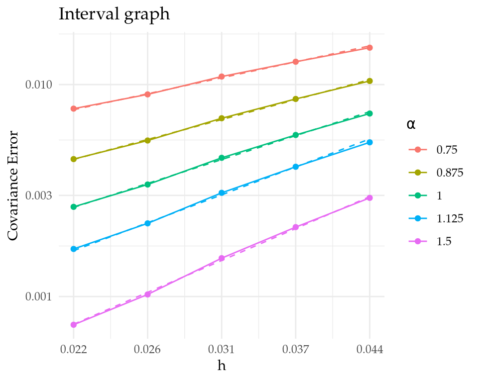

p.interval

Figure 1: Convergence rates for the interval graph.

Circle graph

Follow this link for more details.

# Matern covariance function
matern.covariance <- function(h, kappa, nu, sigma) {
  if (nu == 1 / 2) {
    C <- sigma^2 * exp(-kappa * abs(h))
  } else {
    C <- (sigma^2 / (2^(nu - 1) * gamma(nu))) *
      ((kappa * abs(h))^nu) * besselK(kappa * abs(h), nu)
  }
  C[h == 0] <- sigma^2
  return(as.matrix(C))
}

# Folded.matern.covariance.1d
folded.matern.covariance.1d.local <- function(x, kappa, nu, sigma, L = 1, N = 10, boundary = c("neumann",
                                                                                               "dirichlet", "periodic")) {
  boundary <- tolower(boundary[1])
  if (!(boundary %in% c("neumann", "dirichlet", "periodic"))) {
    stop("The possible boundary conditions are 'neumann',
    'dirichlet' or 'periodic'!")
  }
  addi = t(outer(x, x, "+"))
  diff = t(outer(x, x, "-"))
  s1 <- sapply(-N:N, function(j) { # s1 is a matrix of size length(h)x(2N+1)
    diff + 2 * j * L
  })
  s2 <- sapply(-N:N, function(j) {
    addi + 2 * j * L
  })
  if (boundary == "neumann") {
    C <- rowSums(matern.covariance(h = s1, kappa = kappa,
                                   nu = nu, sigma = sigma) +
                   matern.covariance(h = s2, kappa = kappa,
                                     nu = nu, sigma = sigma))
  } else if (boundary == "dirichlet") {
    C <- rowSums(matern.covariance(h = s1, kappa = kappa,
                                   nu = nu, sigma = sigma) -
                   matern.covariance(h = s2, kappa = kappa,
                                     nu = nu, sigma = sigma))
  } else {
    C <- rowSums(matern.covariance(h = s1,
                                   kappa = kappa, nu = nu, sigma = sigma))
  }
  return(matrix(C, nrow = length(x)))
}

# Function to get the true covariance matrix
gets_true_cov_mat = function(graph, kappa, nu, sigma, N, boundary){
  h = c(0,graph$get_edge_lengths()[1]*graph$mesh$PtE[,2])
  true_cov_mat = folded.matern.covariance.1d.local(x = h, kappa = kappa, nu = nu, sigma = sigma, N = N, boundary = boundary)
  return(true_cov_mat)
}

# Define the graph
r <- 1/(pi)
theta <- seq(from = -pi, to = pi, length.out = 100)
edge <- cbind(1+r+r*cos(theta), r*sin(theta))
edges <- list(edge)
graph <- metric_graph$new(edges = edges)

# parameters
h.ok <- 2^-10
type <- "covariance"
type_rational_approximation = "brasil"
rho <- 0.5
#m = 4
sigma <- 1
N.folded <- 10
boundary <- "periodic" # Do not change this

# Mesh sizes
h_aux <- seq(5.5, 4.5, by = -1/4)
h_vector <- 2^-h_aux
h_label <- paste0("2^-", h_aux, "")
h_label_latex <- sprintf("$2^{-%f}$", h_aux)

# Beta values
alpha_aux <- c(6, 7, 8, 9, 12)
alpha_vector <- alpha_aux/8
alpha_label <- paste0(alpha_aux, "/8")
theoretical_rate <- pmin(2*alpha_vector-1/2,2)

graph.ok <- graph$clone()
# Build graph with overkill mesh
graph.ok$build_mesh(h = h.ok)
graph.ok$compute_fem()

# Get the overkill mesh locations
loc.ok <- graph.ok$mesh$VtE # or graph.ok$get_mesh_locations()

# Initialize the list of graphs and the list of projection matrices
graphs <- list()
A <- list()
for(i in 1:length(h_vector)){
  graphs[[i]] <- graph$clone()
  graphs[[i]]$build_mesh(h = h_vector[i])
  A[[i]] <- graphs[[i]]$fem_basis(loc.ok)
}

cov.error.circle <- matrix(NA, nrow = length(h_vector), ncol = length(alpha_vector))

m_values <- c()
for (j in 1:length(alpha_vector)) {
  alpha <- alpha_vector[j]
  fract_alpha <- alpha - floor(alpha)
  nu <- alpha - 0.5
  kappa <- sqrt(8*nu)/rho
  tau <- sqrt(gamma(nu) / (sigma^2 * kappa^(2*nu) * (4*pi)^(1/2) * gamma(nu + 1/2)))  #sigma = 1, d = 1

  Sigma.true.circle <- gets_true_cov_mat(graph = graph.ok, 
                               kappa = kappa,
                               nu = nu,
                               sigma = sigma,
                               N = N.folded,
                               boundary = boundary)

  for (i in 1:length(h_vector)) {
    h <- h_vector[i]
    m <- min(20, 5*ceiling((min(2*alpha - 1/2,2) + 1/2)^2*log(h)^2/(4*pi^2*fract_alpha)))
    m_values <- c(m_values, m)

    Sigma <- matern.operators(alpha = alpha,  
                             kappa = kappa,
                             tau = tau,
                             m = m,
                             graph = graphs[[i]],
                             type = type,
                             type_rational_approximation = type_rational_approximation)$covariance_mesh()

    Sigma.approx.circle <- A[[i]]%*%Sigma%*%t(A[[i]])

    cov.error.circle[i,j] <- sqrt(as.double(t(graph.ok$mesh$weights)%*%(Sigma.true.circle - Sigma.approx.circle)^2%*%graph.ok$mesh$weights))
  }
}


print(m_values)

##  [1] 10 10  5  5  5 10 10 10  5  5 20 20 20 20 20 20 20 20 20 20 20 20 20 20 20

slope_circle <- numeric(length(alpha_vector))

for (u in 1:length(alpha_vector)) {
  slope_circle[u] <- coef(lm(log(cov.error.circle[,u]) ~ log(h_vector)))[2]
}

transposed_df <- data.frame(t(data.frame(alpha = alpha_vector, theoretical_rate = theoretical_rate, slope = slope_circle)))
rownames(transposed_df) <- c("alpha", "Theoretical rates", "Circle graph")
colnames(transposed_df) <- NULL
# Display the transposed data frame
transposed_df |> paged_table()

loglog_line_equation <- function(x1, y1, slope) {
  b <- log10(y1 / (x1 ^ slope))

  function(x) {
    (x ^ slope) * (10 ^ b)
  }
}

guiding_lines <- matrix(NA, nrow = length(h_vector), ncol = length(alpha_vector))
for (j in 1:length(alpha_vector)) {
  guiding_lines_aux <- matrix(NA, nrow = length(h_vector), ncol = length(h_vector))
  for(k in 1:length(h_vector)){
    point_x1 <- h_vector[k]
    point_y1 <- cov.error.circle[k, j]
    slope <- theoretical_rate[j]
    line <- loglog_line_equation(x1 = point_x1, y1 = point_y1, slope = slope)
    guiding_lines_aux[,k] <- line(h_vector)
  }
  guiding_lines[,j] <- apply(guiding_lines_aux, 1, mean)
}
guiding_lines2 <- guiding_lines

# Generate default ggplot2 colors
default_colors <- scales::hue_pal()(ncol(guiding_lines))

# Create the plot_lines list with different colors for each line
plot_lines <- lapply(1:ncol(guiding_lines), function(i) {
  geom_line(data = data.frame(x = h_vector, y = guiding_lines[, i]),
            aes(x = x, y = y), color = default_colors[i], linetype = "dashed", show.legend = FALSE)
})

df <- as.data.frame(cbind(h_vector, cov.error.circle))
colnames(df) <- c("h_vector", alpha_vector)
df_melted <- melt(df, id.vars = "h_vector", variable.name = "column", value.name = "value")
df_melted2 <- df_melted

p.circle <- ggplot() +
  geom_line(data = df_melted, aes(x = h_vector, y = value, color = column)) +
  geom_point(data = df_melted, aes(x = h_vector, y = value, color = column)) +
  plot_lines +
  labs(title = "Circle graph",
    x = "h",
       y = "Covariance Error",
       color = expression(alpha)) +
  scale_x_log10(breaks = h_vector, labels = round(h_vector,3)) +
  scale_y_log10() +
  theme_minimal() +
  theme(text = element_text(family = "Palatino"))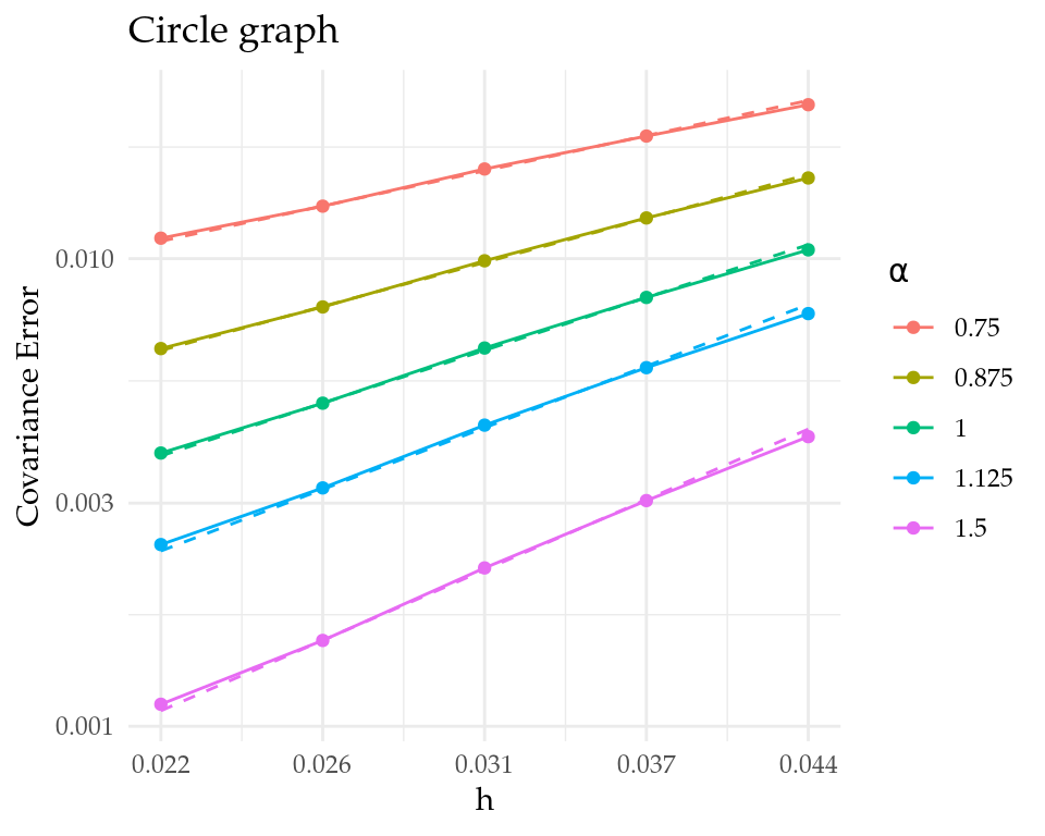

p.circle

Figure 2: Convergence rates for the circle graph.

Tadpole graph

Follow this link for more details.

# Eigenfunctions for the tadpole graph
tadpole.eig <- function(k,graph){
  x1 <- c(0,graph$get_edge_lengths()[1]*graph$mesh$PtE[graph$mesh$PtE[,1]==1,2]) 
  x2 <- c(0,graph$get_edge_lengths()[2]*graph$mesh$PtE[graph$mesh$PtE[,1]==2,2]) 
  
  if(k==0){ 
    f.e1 <- rep(1,length(x1)) 
    f.e2 <- rep(1,length(x2)) 
    f1 = c(f.e1[1],f.e2[1],f.e1[-1], f.e2[-1]) 
    f = list(phi=f1/sqrt(3)) 
    
  } else {
    f.e1 <- -2*sin(pi*k*1/2)*cos(pi*k*x1/2) 
    f.e2 <- sin(pi*k*x2/2)                  
    
    f1 = c(f.e1[1],f.e2[1],f.e1[-1], f.e2[-1]) 
    
    if((k %% 2)==1){ 
      f = list(phi=f1/sqrt(3)) 
    } else { 
      f.e1 <- (-1)^{k/2}*cos(pi*k*x1/2)
      f.e2 <- cos(pi*k*x2/2)
      f2 = c(f.e1[1],f.e2[1],f.e1[-1],f.e2[-1]) 
      f <- list(phi=f1,psi=f2/sqrt(3/2))
    }
  }
  
  return(f)
}


# Function to compute the true covariance matrix
gets_true_cov_mat <- function(graph, kappa, tau, alpha, n.overkill){
  Sigma.kl <- matrix(0,nrow = dim(graph$mesh$V)[1],ncol = dim(graph$mesh$V)[1])
  for(i in 0:n.overkill){
    phi <- tadpole.eig(i,graph)$phi
    Sigma.kl <- Sigma.kl + (1/(kappa^2 + (i*pi/2)^2)^(alpha))*phi%*%t(phi)
    if(i>0 && (i %% 2)==0){ 
      psi <- tadpole.eig(i,graph)$psi
      Sigma.kl <- Sigma.kl + (1/(kappa^2 + (i*pi/2)^2)^(alpha))*psi%*%t(psi)
    }
    
  }
  Sigma.kl <- Sigma.kl/tau^2
  return(Sigma.kl)
}

# Define the graph
edge1 <- rbind(c(0,0), c(1,0))
theta <- seq(from = -pi, to = pi,length.out = 100)
edge2 <- cbind(1+1/pi+cos(theta)/pi, sin(theta)/pi)
edges <- list(edge1, edge2)
graph <- metric_graph$new(edges = edges)

# parameters
h.ok <- 2^-10
type <- "covariance"
type_rational_approximation = "brasil"
rho <- 0.5
#m = 4
sigma <- 1
n.overkill = 1000

# Mesh sizes
h_aux <- seq(5.5, 4.5, by = -1/4)
h_vector <- 2^-h_aux
h_label <- paste0("2^-", h_aux, "")
h_label_latex <- sprintf("$2^{-%f}$", h_aux)

# Beta values
alpha_aux <- c(6, 7, 8, 9, 12)
alpha_vector <- alpha_aux/8
alpha_label <- paste0(alpha_aux, "/8")
theoretical_rate <- pmin(2*alpha_vector-1/2,2)

graph.ok <- graph$clone()
# Build graph with overkill mesh
graph.ok$build_mesh(h = h.ok)
graph.ok$compute_fem()

# Get the overkill mesh locations
loc.ok <- graph.ok$mesh$VtE # or graph.ok$get_mesh_locations()

# Initialize the list of graphs and the list of projection matrices
graphs <- list()
A <- list()
for(i in 1:length(h_vector)){
  graphs[[i]] <- graph$clone()
  graphs[[i]]$build_mesh(h = h_vector[i])
  A[[i]] <- graphs[[i]]$fem_basis(loc.ok)
}

cov.error.tadpole <- matrix(NA, nrow = length(h_vector), ncol = length(alpha_vector))

m_values <- c()
for (j in 1:length(alpha_vector)) {
  alpha <- alpha_vector[j]
  fract_alpha <- alpha - floor(alpha)
  nu <- alpha - 0.5
  kappa <- sqrt(8*nu)/rho
  tau <- sqrt(gamma(nu) / (sigma^2 * kappa^(2*nu) * (4*pi)^(1/2) * gamma(nu + 1/2)))  #sigma = 1, d = 1

  Sigma.true.tadpole <- gets_true_cov_mat(graph = graph.ok,
                               kappa = kappa,
                               tau = tau,
                               alpha = alpha,
                               n.overkill = n.overkill)

  for (i in 1:length(h_vector)) {
    h <- h_vector[i]
    m <- min(20, 5*ceiling((min(2*alpha - 1/2,2) + 1/2)^2*log(h)^2/(4*pi^2*fract_alpha)))
    m_values <- c(m_values, m)

    Sigma <- matern.operators(alpha = alpha,
                             kappa = kappa,
                             tau = tau,
                             m = m,
                             graph = graphs[[i]],
                             type = type,
                             type_rational_approximation = type_rational_approximation)$covariance_mesh()

    Sigma.approx.tadpole <- A[[i]]%*%Sigma%*%t(A[[i]])

    cov.error.tadpole[i,j] <- sqrt(as.double(t(graph.ok$mesh$weights)%*%(Sigma.true.tadpole - Sigma.approx.tadpole)^2%*%graph.ok$mesh$weights))
  }
}

print(m_values)

##  [1] 10 10  5  5  5 10 10 10  5  5 20 20 20 20 20 20 20 20 20 20 20 20 20 20 20

slope_tadpole <- numeric(length(alpha_vector))

for (u in 1:length(alpha_vector)) {
  slope_tadpole[u] <- round(coef(lm(log(cov.error.tadpole[,u]) ~ log(h_vector)))[2], 7)
}

transposed_df <- data.frame(t(data.frame(alpha = alpha_vector, theoretical_rate = theoretical_rate, slope = slope_tadpole)))
rownames(transposed_df) <- c("alpha", "Theoretical rates", "Tadpole graph")
colnames(transposed_df) <- NULL
# Display the transposed data frame
transposed_df |> paged_table()

loglog_line_equation <- function(x1, y1, slope) {
  b <- log10(y1 / (x1 ^ slope))

  function(x) {
    (x ^ slope) * (10 ^ b)
  }
}

guiding_lines <- matrix(NA, nrow = length(h_vector), ncol = length(alpha_vector))
for (j in 1:length(alpha_vector)) {
  guiding_lines_aux <- matrix(NA, nrow = length(h_vector), ncol = length(h_vector))
  for(k in 1:length(h_vector)){
    point_x1 <- h_vector[k]
    point_y1 <- cov.error.tadpole[k, j]
    slope <- theoretical_rate[j]
    line <- loglog_line_equation(x1 = point_x1, y1 = point_y1, slope = slope)
    guiding_lines_aux[,k] <- line(h_vector)
  }
  guiding_lines[,j] <- apply(guiding_lines_aux, 1, mean)
}
guiding_lines3 <- guiding_lines

# Generate default ggplot2 colors
default_colors <- scales::hue_pal()(ncol(guiding_lines))

# Create the plot_lines list with different colors for each line
plot_lines <- lapply(1:ncol(guiding_lines), function(i) {
  geom_line(data = data.frame(x = h_vector, y = guiding_lines[, i]),
            aes(x = x, y = y), color = default_colors[i], linetype = "dashed", show.legend = FALSE)
})

df <- as.data.frame(cbind(h_vector, cov.error.tadpole))
colnames(df) <- c("h_vector", alpha_vector)
df_melted <- melt(df, id.vars = "h_vector", variable.name = "column", value.name = "value")
df_melted3 <- df_melted

p.tadpole <- ggplot() +
  geom_line(data = df_melted, aes(x = h_vector, y = value, color = column)) +
  geom_point(data = df_melted, aes(x = h_vector, y = value, color = column)) +
  plot_lines +
  labs(title = "Tadpole graph",
    x = "h",
       y = "Covariance Error",
       color = expression(alpha)) +
  scale_x_log10(breaks = h_vector, labels = round(h_vector,3)) +
  scale_y_log10() +
  theme_minimal() +
  theme(text = element_text(family = "Palatino"))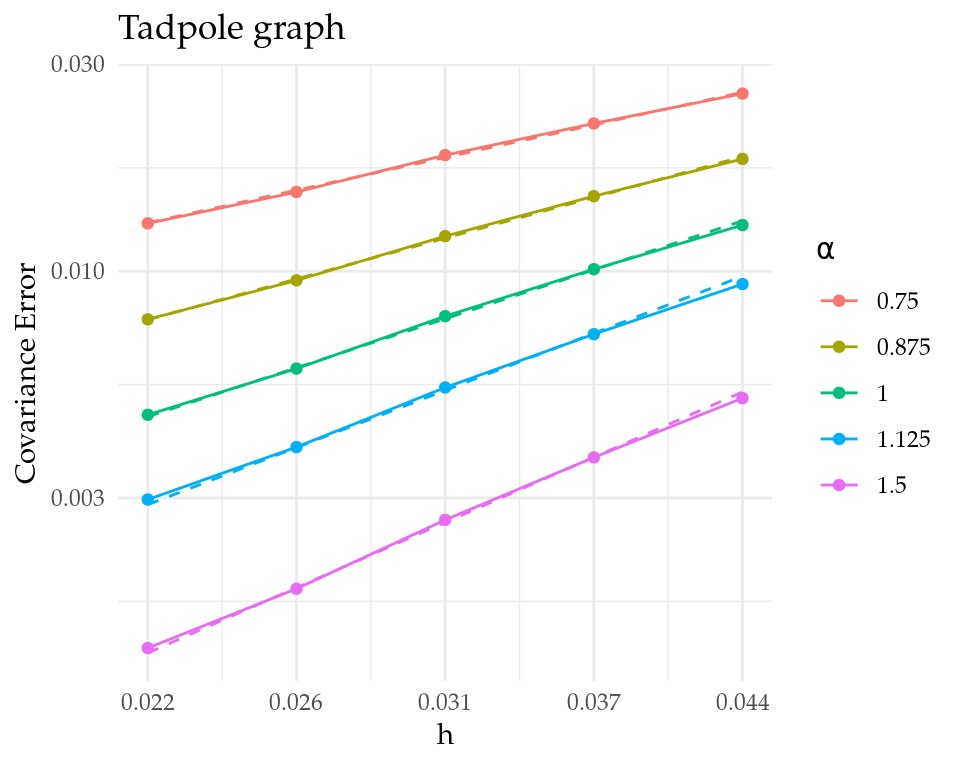

p.tadpole

Figure 3: Convergence rates for the tadpole graph.

Alltogether

transposed_df <- data.frame(t(data.frame(alpha = alpha_vector, 
                                         theoretical_rate = theoretical_rate, 
                                         slope_interval = slope_interval,
                                         slope_circle = slope_circle,
                                         slope_tadpole = slope_tadpole)))
rownames(transposed_df) <- c("alpha", "Theoretical rates", "Interval graph", "Circle graph", "Tadpole graph")
colnames(transposed_df) <- NULL
# Display the transposed data frame
transposed_df |> paged_table()

ff_data <- rbind(mutate(df_melted1, graph = "Intervalgraph"),
                 mutate(df_melted2, graph = "Circlegraph"),
                 mutate(df_melted3, graph = "Tadpolegraph"))

ff_data$graph <- factor(ff_data$graph, levels = c("Intervalgraph", "Circlegraph", "Tadpolegraph"))

glines <- c(as.vector(guiding_lines1), as.vector(guiding_lines2), as.vector(guiding_lines3))
gg_data <- ff_data %>% 
  mutate(value = glines)

graph_labels <- c("Intervalgraph" = "Interval graph", 
                  "Circlegraph" = "Circle graph", 
                  "Tadpolegraph" = "Tadpole graph")

last_plot <- ggplot() + 
  geom_line(data = ff_data, aes(h_vector, value, colour = as.factor(column)), linewidth = 0.7) +
  geom_line(data = gg_data, aes(h_vector, value, colour = as.factor(column)), linetype = "dashed", linewidth = 0.3) +
  geom_point(data = ff_data, aes(h_vector, value, colour = as.factor(column))) +
  facet_grid(~ graph, labeller = as_labeller(graph_labels)) +
  scale_y_log10() +
  scale_x_log10(breaks = h_vector, labels = round(h_vector, 3)) +
  theme_bw() +
  theme(panel.spacing = unit(0.4, "cm"), 
        text = element_text(family = "Palatino"),
        strip.text = element_text(size = 16),        # Panel titles
        axis.title = element_text(size = 14),        # Axis titles
        axis.text = element_text(size = 12),         # Axis text
        legend.title = element_text(size = 14),      # Legend title
        legend.text = element_text(size = 12)) +
  labs(x = "h", y = "Covariance Error", color = bquote(alpha)) 

last_plot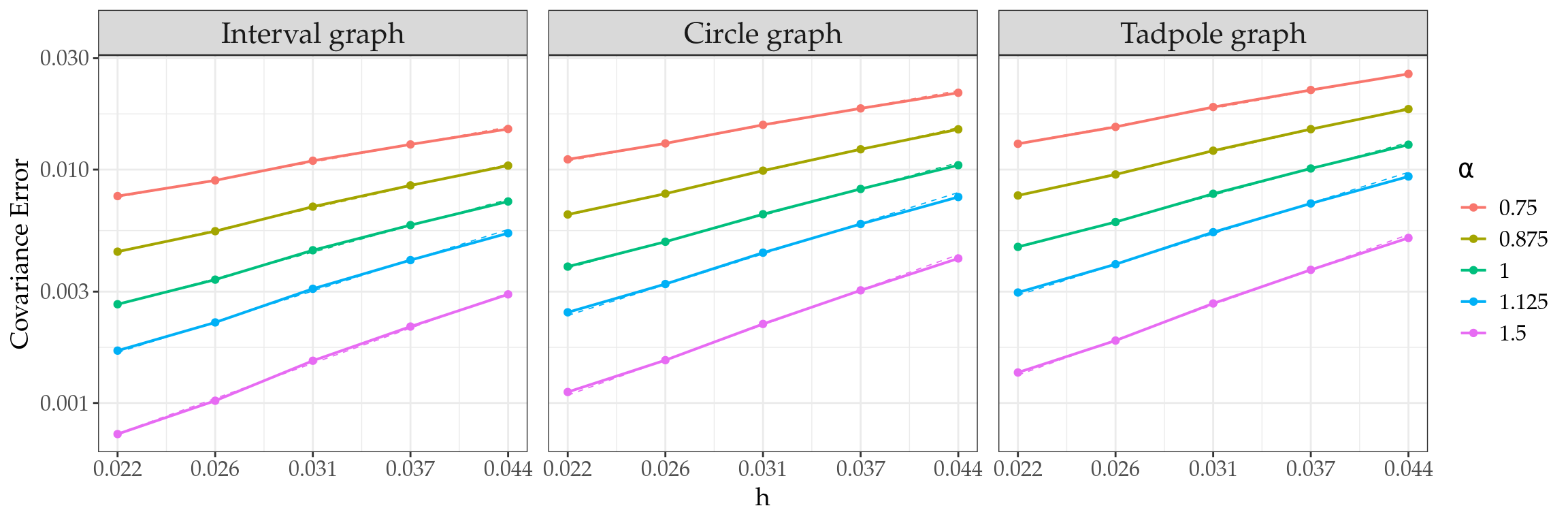

Figure 4: Observed covariance error for different values of \(\alpha\) as functions of the mesh size \(h\).

ggsave(here("data_files/conv_rates_new.png"), width = 12, height = 4, plot = last_plot, dpi = 300)

References

cite_packages(output = "paragraph", out.dir = ".")

We used R version 4.4.1 (R Core Team 2024a) and the following R packages: cowplot v. 1.1.3 (Wilke 2024), ggmap v. 4.0.0.900 (Kahle and Wickham 2013), ggpubr v. 0.6.0 (Kassambara 2023), ggtext v. 0.1.2 (Wilke and Wiernik 2022), grid v. 4.4.1 (R Core Team 2024b), here v. 1.0.1 (Müller 2020), htmltools v. 0.5.8.1 (Cheng et al. 2024), INLA v. 24.12.11 (Rue, Martino, and Chopin 2009; Lindgren, Rue, and Lindström 2011; Martins et al. 2013; Lindgren and Rue 2015; De Coninck et al. 2016; Rue et al. 2017; Verbosio et al. 2017; Bakka et al. 2018; Kourounis, Fuchs, and Schenk 2018), inlabru v. 2.12.0.9002 (Yuan et al. 2017; Bachl et al. 2019), knitr v. 1.48 (Xie 2014, 2015, 2024), latex2exp v. 0.9.6 (Meschiari 2022), Matrix v. 1.6.5 (Bates, Maechler, and Jagan 2024), MetricGraph v. 1.4.0.9000 (Bolin, Simas, and Wallin 2023b, 2023a, 2023c, 2024; Bolin et al. 2024), OpenStreetMap v. 0.4.0 (Fellows and JMapViewer library by Jan Peter Stotz 2023), osmdata v. 0.2.5 (Mark Padgham et al. 2017), patchwork v. 1.2.0 (Pedersen 2024), plotly v. 4.10.4 (Sievert 2020), plotrix v. 3.8.4 (J 2006), reshape2 v. 1.4.4 (Wickham 2007), rmarkdown v. 2.28 (Xie, Allaire, and Grolemund 2018; Xie, Dervieux, and Riederer 2020; Allaire et al. 2024), rSPDE v. 2.4.0.9000 (Bolin and Kirchner 2020; Bolin and Simas 2023; Bolin, Simas, and Xiong 2024), scales v. 1.3.0 (Wickham, Pedersen, and Seidel 2023), sf v. 1.0.19 (E. Pebesma 2018; E. Pebesma and Bivand 2023), sp v. 2.1.4 (E. J. Pebesma and Bivand 2005; Bivand, Pebesma, and Gomez-Rubio 2013), tidyverse v. 2.0.0 (Wickham et al. 2019), viridis v. 0.6.4 (Garnier et al. 2023), xaringanExtra v. 0.8.0 (Aden-Buie and Warkentin 2024).

Aden-Buie, Garrick, and Matthew T. Warkentin. 2024. xaringanExtra: Extras and Extensions for “xaringan” Slides. https://CRAN.R-project.org/package=xaringanExtra.

Allaire, JJ, Yihui Xie, Christophe Dervieux, Jonathan McPherson, Javier Luraschi, Kevin Ushey, Aron Atkins, et al. 2024. rmarkdown: Dynamic Documents for r. https://github.com/rstudio/rmarkdown.

Bachl, Fabian E., Finn Lindgren, David L. Borchers, and Janine B. Illian. 2019. “inlabru: An R Package for Bayesian Spatial Modelling from Ecological Survey Data.” Methods in Ecology and Evolution 10: 760–66. https://doi.org/10.1111/2041-210X.13168.

Bakka, Haakon, Håvard Rue, Geir-Arne Fuglstad, Andrea I. Riebler, David Bolin, Janine Illian, Elias Krainski, Daniel P. Simpson, and Finn K. Lindgren. 2018. “Spatial Modelling with INLA: A Review.” WIRES (Invited Extended Review) xx (Feb): xx–. http://arxiv.org/abs/1802.06350.

Bates, Douglas, Martin Maechler, and Mikael Jagan. 2024. Matrix: Sparse and Dense Matrix Classes and Methods. https://CRAN.R-project.org/package=Matrix.

Bivand, Roger S., Edzer Pebesma, and Virgilio Gomez-Rubio. 2013. Applied Spatial Data Analysis with R, Second Edition. Springer, NY. https://asdar-book.org/.

Bolin, David, and Kristin Kirchner. 2020. “The Rational SPDE Approach for Gaussian Random Fields with General Smoothness.” Journal of Computational and Graphical Statistics 29 (2): 274–85. https://doi.org/10.1080/10618600.2019.1665537.

Bolin, David, Mihály Kovács, Vivek Kumar, and Alexandre B. Simas. 2024. “Regularity and Numerical Approximation of Fractional Elliptic Differential Equations on Compact Metric Graphs.” Mathematics of Computation 93 (349): 2439–72. https://doi.org/10.1090/mcom/3929.

Bolin, David, and Alexandre B. Simas. 2023. rSPDE: Rational Approximations of Fractional Stochastic Partial Differential Equations. https://CRAN.R-project.org/package=rSPDE.

Bolin, David, Alexandre B. Simas, and Jonas Wallin. 2023a. “Markov Properties of Gaussian Random Fields on Compact Metric Graphs.” arXiv Preprint arXiv:2304.03190. https://doi.org/10.48550/arXiv.2304.03190.

———. 2023b. MetricGraph: Random Fields on Metric Graphs. https://CRAN.R-project.org/package=MetricGraph.

———. 2023c. “Statistical Inference for Gaussian Whittle-Matérn Fields on Metric Graphs.” arXiv Preprint arXiv:2304.10372. https://doi.org/10.48550/arXiv.2304.10372.

———. 2024. “Gaussian Whittle-Matérn Fields on Metric Graphs.” Bernoulli 30 (2): 1611–39. https://doi.org/10.3150/23-BEJ1647.

Bolin, David, Alexandre B. Simas, and Zhen Xiong. 2024. “Covariance-Based Rational Approximations of Fractional SPDEs for Computationally Efficient Bayesian Inference.” Journal of Computational and Graphical Statistics 33 (1): 64–74. https://doi.org/10.1080/10618600.2023.2231051.

Cheng, Joe, Carson Sievert, Barret Schloerke, Winston Chang, Yihui Xie, and Jeff Allen. 2024. htmltools: Tools for HTML. https://CRAN.R-project.org/package=htmltools.

De Coninck, Arne, Bernard De Baets, Drosos Kourounis, Fabio Verbosio, Olaf Schenk, Steven Maenhout, and Jan Fostier. 2016. “Needles: Toward Large-Scale Genomic Prediction with Marker-by-Environment Interaction.” Genetics 203 (1): 543–55. https://doi.org/10.1534/genetics.115.179887.

Fellows, Ian, and using the JMapViewer library by Jan Peter Stotz. 2023. OpenStreetMap: Access to Open Street Map Raster Images. https://CRAN.R-project.org/package=OpenStreetMap.

Garnier, Simon, Ross, Noam, Rudis, Robert, Camargo, et al. 2023. viridis(Lite) - Colorblind-Friendly Color Maps for r. https://doi.org/10.5281/zenodo.4679423.

J, Lemon. 2006. “Plotrix: A Package in the Red Light District of r.” R-News 6 (4): 8–12.

Kahle, David, and Hadley Wickham. 2013. “ggmap: Spatial Visualization with Ggplot2.” The R Journal 5 (1): 144–61. https://journal.r-project.org/archive/2013-1/kahle-wickham.pdf.

Kassambara, Alboukadel. 2023. ggpubr: “ggplot2” Based Publication Ready Plots. https://CRAN.R-project.org/package=ggpubr.

Kourounis, D., A. Fuchs, and O. Schenk. 2018. “Towards the Next Generation of Multiperiod Optimal Power Flow Solvers.” IEEE Transactions on Power Systems PP (99): 1–10. https://doi.org/10.1109/TPWRS.2017.2789187.

Lindgren, Finn, and Håvard Rue. 2015. “Bayesian Spatial Modelling with R-INLA.” Journal of Statistical Software 63 (19): 1–25. http://www.jstatsoft.org/v63/i19/.

Lindgren, Finn, Håvard Rue, and Johan Lindström. 2011. “An Explicit Link Between Gaussian Fields and Gaussian Markov Random Fields: The Stochastic Partial Differential Equation Approach (with Discussion).” Journal of the Royal Statistical Society B 73 (4): 423–98.

Mark Padgham, Bob Rudis, Robin Lovelace, and Maëlle Salmon. 2017. “Osmdata.” Journal of Open Source Software 2 (14): 305. https://doi.org/10.21105/joss.00305.

Martins, Thiago G., Daniel Simpson, Finn Lindgren, and Håvard Rue. 2013. “Bayesian Computing with INLA: New Features.” Computational Statistics and Data Analysis 67: 68–83.

Meschiari, Stefano. 2022. Latex2exp: Use LaTeX Expressions in Plots. https://CRAN.R-project.org/package=latex2exp.

Müller, Kirill. 2020. here: A Simpler Way to Find Your Files. https://CRAN.R-project.org/package=here.

Pebesma, Edzer. 2018. “Simple Features for R: Standardized Support for Spatial Vector Data.” The R Journal 10 (1): 439–46. https://doi.org/10.32614/RJ-2018-009.

Pebesma, Edzer J., and Roger Bivand. 2005. “Classes and Methods for Spatial Data in R.” R News 5 (2): 9–13. https://CRAN.R-project.org/doc/Rnews/.

Pebesma, Edzer, and Roger Bivand. 2023. Spatial Data Science: With applications in R. Chapman and Hall/CRC. https://doi.org/10.1201/9780429459016.

Pedersen, Thomas Lin. 2024. patchwork: The Composer of Plots. https://CRAN.R-project.org/package=patchwork.

R Core Team. 2024a. R: A Language and Environment for Statistical Computing. Vienna, Austria: R Foundation for Statistical Computing. https://www.R-project.org/.

———. 2024b. R: A Language and Environment for Statistical Computing. Vienna, Austria: R Foundation for Statistical Computing. https://www.R-project.org/.

Rue, Håvard, Sara Martino, and Nicholas Chopin. 2009. “Approximate Bayesian Inference for Latent Gaussian Models Using Integrated Nested Laplace Approximations (with Discussion).” Journal of the Royal Statistical Society B 71: 319–92.

Rue, Håvard, Andrea I. Riebler, Sigrunn H. Sørbye, Janine B. Illian, Daniel P. Simpson, and Finn K. Lindgren. 2017. “Bayesian Computing with INLA: A Review.” Annual Reviews of Statistics and Its Applications 4 (March): 395–421. http://arxiv.org/abs/1604.00860.

Sievert, Carson. 2020. Interactive Web-Based Data Visualization with r, Plotly, and Shiny. Chapman; Hall/CRC. https://plotly-r.com.

Verbosio, Fabio, Arne De Coninck, Drosos Kourounis, and Olaf Schenk. 2017. “Enhancing the Scalability of Selected Inversion Factorization Algorithms in Genomic Prediction.” Journal of Computational Science 22 (Supplement C): 99–108. https://doi.org/10.1016/j.jocs.2017.08.013.

Wickham, Hadley. 2007. “Reshaping Data with the reshape Package.” Journal of Statistical Software 21 (12): 1–20. http://www.jstatsoft.org/v21/i12/.

Wickham, Hadley, Mara Averick, Jennifer Bryan, Winston Chang, Lucy D’Agostino McGowan, Romain François, Garrett Grolemund, et al. 2019. “Welcome to the tidyverse.” Journal of Open Source Software 4 (43): 1686. https://doi.org/10.21105/joss.01686.

Wickham, Hadley, Thomas Lin Pedersen, and Dana Seidel. 2023. scales: Scale Functions for Visualization. https://CRAN.R-project.org/package=scales.

Wilke, Claus O. 2024. cowplot: Streamlined Plot Theme and Plot Annotations for “ggplot2”. https://CRAN.R-project.org/package=cowplot.

Wilke, Claus O., and Brenton M. Wiernik. 2022. ggtext: Improved Text Rendering Support for “ggplot2”. https://CRAN.R-project.org/package=ggtext.

Xie, Yihui. 2014. “knitr: A Comprehensive Tool for Reproducible Research in R.” In Implementing Reproducible Computational Research, edited by Victoria Stodden, Friedrich Leisch, and Roger D. Peng. Chapman; Hall/CRC.

———. 2015. Dynamic Documents with R and Knitr. 2nd ed. Boca Raton, Florida: Chapman; Hall/CRC. https://yihui.org/knitr/.

———. 2024. knitr: A General-Purpose Package for Dynamic Report Generation in r. https://yihui.org/knitr/.

Xie, Yihui, J. J. Allaire, and Garrett Grolemund. 2018. R Markdown: The Definitive Guide. Boca Raton, Florida: Chapman; Hall/CRC. https://bookdown.org/yihui/rmarkdown.

Xie, Yihui, Christophe Dervieux, and Emily Riederer. 2020. R Markdown Cookbook. Boca Raton, Florida: Chapman; Hall/CRC. https://bookdown.org/yihui/rmarkdown-cookbook.

Yuan, Yuan, Bachl, Fabian E., Lindgren, Finn, Borchers, et al. 2017. “Point Process Models for Spatio-Temporal Distance Sampling Data from a Large-Scale Survey of Blue Whales.” Ann. Appl. Stat. 11 (4): 2270–97. https://doi.org/10.1214/17-AOAS1078.